Learn R | 日期时间处理之lubridate包

用过R的朋友们相信一定不会对Hadley·Wickham这个名字有所陌生，作为RStudio的Chief Scientist，他为R用户贡献了多个重量级的package（ggplot2、dplyr等等）。而今天介绍的这个lubridate包，也是由他所编写，专注于对日期时间数据（Date-time data）的处理。

对于日期时间数据，R在基础包中提供了两种类型的时间数据，一类是Date日期数据，它不包括时间和时区信息；另一类是POSIXct/POSIXlt类型数据，其中包括了日期、时间和时区信息。一般来讲，R语言中建立时序数据是通过字符型转化而来，但由于时序数据形式多样，而且R中存贮格式也是五花八门，例如Date/ts/xts/zoo/tis/fts等等。用户很容易被一系列的数据格式所迷惑，所以时序数据的转化和操作并不是非常方便。

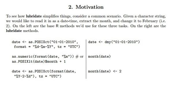
为此，我们引入第三方包lubridate，该包主要有两类函数，一类用于处理时点数据（time instants），另一类则用于处理时段数据（time spans）。虽然这些基础功能R Base也能实现，但实现方式及其繁琐，通过下图的对比，我们可以看到同样是时间数据处理，lubridate包比R的基础包的操作是何等的简洁。

一、解析日期与时间（Parsing dates and times）

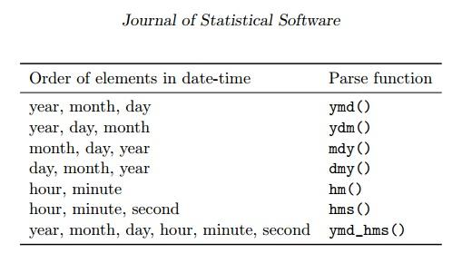
首先，在使用lubridate包识别日期前，我们需要告诉它年（y）月（m）日（d）的排列顺序，而函数本身就是这几个字母的组合，非常形象：

> ymd(20170629);myd(06201729);dmy(29062017)
[1] "2017-06-29"
[1] "2017-06-29"
[1] "2017-06-29"

在此基础上，如果需要读取含具体时间的数据，就需要在函数里再加上小时（h）分钟（m）和秒（s）；如果需要读入的时间具有特定时区，那就用tz选项来指定。

> test_date <- ymd_hms("2017-06-29-12-01-30", tz = "Pacific/Auckland")
> test_date
[1] "2017-06-29 12:01:30 NZST"

所有公式如下表：

lubriadate非常灵活，它可以“智能”的判断我们的输入格式，最好的得到标准的时间格式，甚至即使你的输入不完全，通过一个truncated选项，也可以识别不完整信息的日期输入格式。

> test_date<- c(20170601, "2017-06-02", "2017 06 03", "2017-6-4","2017-6, 5", "Created on 2017 6 6", "201706 !!! 07")
> ymd(test_date)
[1] "2017-06-01" "2017-06-02" "2017-06-03" "2017-06-04" "2017-06-05" "2017-06-06" "2017-06-07"

在上面的这个例子中，日期时间数据虽然杂乱，但还是按照年、月、日的顺序排列的，但如果拿到的数据年月日是无序排列的呢？

这里就需要介绍一个新的函数parse_date_time()，它可以将格式各样的日期时间字符转换为日期时间类型的数据。该函数中有一个重要的参数，即orders，通过该参数指定可能的日期格式顺序，如年-月-日或月-日-年等顺序。

> test_date <- c('20131113','120315','12/17/1996','09-01-01','2015 12 23','2009-1, 5','Created on 2013 4 6')
> parse_date_time(test_date,order = c('ymd','mdy','dmy','ymd'))
[1] "2013-11-13 UTC" "2012-03-15 UTC" "1996-12-17 UTC" "2009-01-01 UTC" "2015-12-23 UTC"
[6] "2009-01-05 UTC" "2013-04-06 UTC"

二、设置与提取信息（Setting and Extracting information）

1. 精确提取

从日期时间提取信息的函数也非常直观，second()，minute()，hour()，day()，wday()，yday()，week()，month()，year()，tz()分别可以提取秒，分，小时，天，周的第几天，年的第几天，星期，月，年和时区的信息。

这些函数同样也可以用来设置修改这些信息。其中，wday()和month()这两个功能有一个label的选项，可以选择显示数值或是名字（eg：wday()可显示7或者Sat。注：weekday默认周日为1）

> test <- ymd_hms('2017/06/29/12/00/00')
> test
[1] "2017-06-29 12:00:00 UTC"
> second(test) <- 30
> test
[1] "2017-06-29 12:00:30 UTC"

> wday(test)
[1] 5
> wday(test,label = TRUE)
[1] Thurs
Levels: Sun < Mon < Tues < Wed < Thurs < Fri < Sat

2. 模糊提取（取整）

模糊取整即截断函数，即将日期时间型数据取整到不同的单位，如年、季、月、日、时等。

# 四舍五入取整
> round_date()
# 向下取整
> floor_date()
# 向上取整
> ceiling_date()

> test_date <- as.POSIXct("2017-06-29 12:34:59")
> round_date(test_date,'hour')
[1] "2017-06-29 13:00:00 CST"
> ceiling_date(test_date,'hour')
[1] "2017-06-29 13:00:00 CST"
> floor_date(test_date,'hour')
[1] "2017-06-29 12:00:00 CST"

# 自定义提取
> x <- as.POSIXct("2017-06-29 12:01:59.23")
> round_date(x, "second")
[1] "2017-06-29 12:01:59 CST"
> round_date(x, "minute")
[1] "2017-06-29 12:02:00 CST"
> round_date(x, "2 hours")
[1] "2017-06-29 12:00:00 CST"
> round_date(x, "halfyear")
[1] "2017-07-01 CST"
> round_date(x, "month")
[1] "2017-07-01 CST"
> round_date(x, "5 mins")
[1] "2017-06-29 12:00:00 CST"
# 向上向下取整同理

三、时区（Time Zones）

在lubridate包中，与时区相关的function主要做两件事。其一，显示同一个时间点在不同时区的时间；其二，结合某个时间点和给定时区，新建一个给定时区的时间点。简单来讲第一个是变换时区，用with_tz()；第二个是固定时区，用force_tz()。

> test_date <- ymd_hms("2017-06-29 09:00:00", tz = "Pacific/Auckland")
> with_tz(test_date,"America/New_York")
[1] "2017-06-28 17:00:00 EDT"

# 给定时间和时区，新建一个给定时区的对应时间点
> test_date <- ymd_hms("2017-06-29 12:00:00", tz = "America/Chicago")
> test_date
[1] "2017-06-29 12:00:00 CDT"
> test_date_1 <- force_tz(test_date,tz="Europe/London")
> test_date_1
[1] "2017-06-29 12:00:00 BST"

四、时间间隔（Time Intervals）

> begin1 <- ymd_hms("20150903,12:00:00")
> end1 <- ymd_hms("20160804,12;30:00")
> begin2 <- ymd_hms("20151203,12:00:00")
> end2 <- ymd_hms("20160904,12;30:00")

> test_date_1 <- interval(begin1,end1)
> test_date_1
[1] 2015-09-03 12:00:00 UTC--2016-08-04 12:30:00 UTC
> test_date_2 <- interval(begin2,end2)
# 判断两段时间是否有重叠
> int_overlaps(test_date_1,test_date_2)
[1] TRUE

其他操作时间间隔的函数还包括：int_start，int_end，int_flip，int_shift，int_aligns，union，intersect和%within%等。

在得到时间间隔的数据后，我们还可以通过time_length()函数进一步计算间隔内的不同度量单位下的时间：

> time_length(test_date_1,'day')
[1] 336.0208
> time_length(test_date_1,'year')
[1] 0.9180897
> time_length(test_date_1,'month')
[1] 11.03293
> time_length(test_date_1,'seconds')
[1] 29032200

五、日期时间的计算（Arithmetic with date times）

1. 时间跨度（durations和periods）

时间间隔是特定的时间跨度（因为它绑定在特定时间点上）。lubridate同时也提供了一般的时间跨度的类：durations和periods。建立periods的function是用时间单位（复数）来命名的。而建立duration的function命名和periods的一致，仅在前缀加一个‘d'。

# periods
> minutes(1)   
[1] "1M 0S"
# durations[加前缀'd']
> dminutes(1)  
[1] "60s"

为什么要这两个不同的类呢？因为时间线（timeline）并没有数字线（number line）那样可靠。durations类通常提供了更准确的运算结果。一个duration年总是等于365天。而periods是随着时间线的波动而给出更理性的结果，这一特点在建立时钟时间（clock times）的模型时非常有用。比方说，durations遇到闰年时，结果就太死板，而periods给出的结果就灵活很多：

> leap_year(2016)
[1] TRUE
> ymd(20160101)+years(1)
[1] "2017-01-01"
> ymd(20160101)+dyears(1)
[1] "2016-12-31"

我们可以用periods或者durations来做基本的日期运算。例如：得出接下来的六周的一个相同时间点：

> test_date <- test_date + weeks(0:5)
> test_date
[1] "2017-06-29 12:00:00 CDT" "2017-07-06 12:00:00 CDT" "2017-07-13 12:00:00 CDT"
[4] "2017-07-20 12:00:00 CDT" "2017-07-27 12:00:00 CDT" "2017-08-03 12:00:00 CDT"

> test_date_2 / ddays(1)
[1] 276.0208
> test_date_2 / dminutes(5)
[1] 79494

# 取整
> test_date_2 %/% months(1)
[1] 9
# 取余
> test_date_2 %% months(1)
[1] 2016-09-03 12:00:00 UTC--2016-09-04 12:30:00 UTC

用时间间隔为模数会得到一个余数，它是一个新的时间间隔。可以用as.period()把这个时间间隔转变为period类（非特定时间跨度的类）。

> as.period(test_date_2 %% months(1))
[1] "1d 0H 30M 0S"

2. %m+%

在时间计算时，由于日期数据的特殊性，如果我们需要得到每个月的最后一天的日期数据，直接在某一个月的最后一天上加上月份很明显是错误的。为此我们引入%m+%函数：

> test_date_0 <- as.Date('2015-01-31')
> test_date_2 <- test_date_0 %m+% months(0:11)
> test_date_2
 [1] "2015-01-31" "2015-02-28" "2015-03-31" "2015-04-30" "2015-05-31" "2015-06-30"
 [7] "2015-07-31" "2015-08-31" "2015-09-30" "2015-10-31" "2015-11-30" "2015-12-31"