Shader相册第6期 --- 实时水面模拟与渲染(一)

音速键盘猫

大萌猫 >_<

写在前面

专栏断更了大半年. 这段时间里先经历了小腿骨折, 又经历了腾讯实习. 如今因必修课返校才抽出时间整理和分享. 从现在开始到过年前我会保证更新频率.

本篇主要介绍水面运动的基本模拟. 后面的文章中我会逐步介绍各种水面的渲染和针对特殊运动的处理.

本文会由浅入深讲解实时水面模拟技术, 最后获得如下的模拟结果:

主要内容一览

Gerstner(Trochoidal) Wave
Phillips Spectrum
基于GPU的快速傅立叶变换
海面浪端白沫(Whitecap)检测

引入 - Sinusoid正弦波

图形学中, 水面的运动模拟可以分成两个方面: 网格的几何波动与法线计算. 我们知道最简单的振动是简谐振动, 其波形为正弦波. 多个简谐振动叠加即可以产生非常复杂的振动波形, 因此可以使用正弦波来模拟水面的波动.

对于某一特定的正弦波, 我们有:

W(x, z, t) = A \times sin(D \cdot (x, z) \times \omega + t \times\varphi)

其中, (x, z) 代表水平面上的位置, t 代表时间, A 代表振幅, D 代表运动方向, \omega 代表频率, \varphi 代表相位.

对于多个正弦波叠加产生的波形, 我们有:

H(x, z ,t) = \sum_{}^{}{(A_{i} \times sin(D_{i} \cdot (x, z) \times \omega_{i} + t \times \varphi_{i}))}

即: 针对一组振幅, 方向, 频率与相位的数据, 我们能够生成一组对应的正弦波. 这些正弦波叠加后我们即可得到一个关于水平面位置和时间的高度函数. 在点元着色器中计算高度函数, 并用于修改原始顶点的Y坐标即可实现网格的几何波动.

到此为止, 水面运动模拟的第一个部分已经完成, 现在我们需要得到每一个顶点的法线:

N(x, z) = \bigl(-\frac{\partial}{\partial x}(H(x, z, t)), 1 ,-\frac{\partial}{\partial z}(H(x, z, t))\bigr)

\frac{\partial}{\partial x}\bigl(H(x, z, t)\bigr) = \sum_{}^{}{} \Bigl(\omega_{i} \times \ D_{i} \times A_{i} \times cos\bigl(D_{i} \cdot (x, z) \times \omega_{i} + t \times \varphi_{i}\bigr)\Bigr)

由于篇幅所限本文不列出具体的推导过程, 感兴趣的读者可以前往GPU Gems [1] 一探究竟.

确定了网格上每一个顶点的坐标和法线后, 即可得到下图的模拟结果:

进化 - Gerstner Wave与其实现

使用正弦波模拟能够得到一个平滑的叠加波形, 非常适合于模拟平静的水面, 比如湖面和池塘等. 但是当风浪较大, 水较深时, 波峰会显得更加尖锐, 波谷会更宽阔而平滑.

单纯使用正弦波叠加无法实现这样的"陡峭"效果, 因此我们需要使用新的模拟模型 -- Gerstner Wave [2].

流体动力学中, Gerstner Wave是周期重力波欧拉方程的解, 其描述的是拥有无限深度且不可压缩的流体表面的波形. 下面放一张动图, 让读者能对Gerstner Wave有一个更加清晰直观的了解:

Gerstner Wave的解如下:

P(x, z, t)=\left( \begin{aligned} & x + \sum \biggl( Q_{i}A_{i} \times D_{i}.x \times cos \bigl( \ \omega_{i}D_{i} \cdot (x, z) + \varphi_{i}t\bigr)\biggr) \\ & \sum \biggl( A_{i}sin\bigl(\omega_{i}D_{i} \cdot (x, z) + t\varphi_{i}\bigr)\biggr)\\ & z + \sum \biggl( Q_{i}A_{i} \times D_{i}.z \times cos \bigl( \ \omega_{i}D_{i} \cdot (x, z) + \varphi_{i}t\bigr)\biggr) \\ \end{aligned} \right).

其中, Q 代表的是波形的尖锐程度. 经过观察发现, 如果 Q 为0, 那么Gerstner Wave就退化成了正弦波. 不过值得注意的是, Q_{i} = \frac{1}{\omega_{i}A_{i}} 时, 该Gerstner Wave的波峰达到最尖锐的程度. 如果 Q_{i} > \frac{1}{\omega_{i}A_{i}} , 网格顶点会因左右运动幅度过大而形成穿插.

接下来我们考虑法线. 对于法线我们有如下公式:

N(x, z, t)=\left( \begin{aligned} &- \sum \biggl( D_{i}.x \times \omega_{i} \times A_{i} \times cos(\omega_{i} \times D_{i} \cdot P + t\varphi) \biggr) \\ & 1- \sum \biggl( Q_{i} \times \omega_{i} \times A_{i} \times sin(\omega_{i} \times D_{i} \cdot P + t\varphi) \biggr) \\ &- \sum \biggl( D_{i}.z \times \omega_{i} \times A_{i} \times cos(\omega_{i} \times D_{i} \cdot P + t\varphi) \biggr) \\ \end{aligned} \right).

本例中使用了5个波形叠加, 应用顶点位置与法线后再加上Tessellation得到的结果如下:

我这里将振幅等数据作为"倍数"考虑, 因此得到的着色器代码如下:

inline void GerstnerLevelOne(out half3 offsets, out half3 normal, half3 vertex, half3 sVertex, 
							half amplitude, half frequency, half steepness, half speed,
							half4 directionAB, half4 directionCD)
{
	half3 offs = 0;

	for(int i = 0;i < 5;i++)
	{
		offs.x += steepness * amplitude * steeps[i] * amps[i] * dir[i].x * cos(frequency * fs[i] * dot(sVertex.xz, dir[i]) + speeds[i] * frequency * fs[i] * _Time.y);
		offs.z += steepness * amplitude * steeps[i] * amps[i] * dir[i].y * cos(frequency * fs[i] * dot(sVertex.xz, dir[i]) + speeds[i] * frequency * fs[i] * _Time.y);
		offs.y += amplitude * amps[i] * sin(frequency * fs[i] * dot(sVertex.xz, dir[i].xy) + speeds[i] * frequency * fs[i] * _Time.y);
	}

	offsets = offs;

	normal = half3(0, 1, 0);
	for(int i = 0;i < 5;i++)
	{
		normal.x -= dir[i].x * frequency * fs[i] * amplitude * amps[i] * cos(dot(offs, frequency * fs[i] * dir[i]) + speeds[i] * frequency * fs[i] * _Time.y);
		normal.z -= dir[i].y * frequency * fs[i] * amplitude * amps[i] * cos(dot(offs, frequency * fs[i] * dir[i]) + speeds[i] * frequency * fs[i] * _Time.y);
		normal.y -= steepness * steeps[i] * frequency * fs[i] * amps[i] * amplitude * sin(dot(offs, frequency * fs[i] * dir[i]) + speeds[i] * frequency * fs[i] * _Time.y);
	}
}

Gerstner Wave在游戏中比较常用. 网络上有一个UE4的实现教程 [3], 写得非常好, 大家可以参考一下.

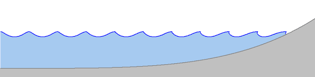
Gerstner Wave还有一个变种 --- Skewed Trochoidal Wave, 可以用来模拟涌向岸边的潮水. 其原理可以在这里了解(似乎需要梯子).

介绍 - 海洋学统计模型

海洋科学中并不使用Gerstner Wave作为海面模拟方案, 而是使用基于经验推导出的统计学模型 [4]:

h(x, t) =\sum_{k}\tilde{h}(k, t)exp(ik \cdot x)

k = (2\pi n / L_{x}, 2\pi m / L_{z})

其中, n, m 可以理解为网格中每一个顶点的横向和纵向索引, 而求解高度函数 h 只需要对 \tilde{h}(k, t) 做傅立叶变换即可. \tilde{h}(k, t) 定义如下:

\tilde{h}(k, t) = \tilde{h}_{0}exp\{i\omega(k)t\} + \tilde{h}_{0}^{*}exp\{-i\omega(k)t\}

\tilde{h}_{0}(k) = (\xi_{r} + i\xi_{i})\sqrt{P(k) / 2}

\omega^{2}(k) = gk(1 + k^{2}L^{2})

其中, \xi_{r} 和 \xi_{i} 是0-1之间的随机数, 不同分布形式的随机数会导致不同的海洋模拟结果; P(k) 是初始频谱, 本篇文章中我们使用Phillips频谱:

P_{h}(k) = A \frac{exp\bigl( -1 / (kL)^{2} \bigr)}{k^{4}}|\bar{k} \cdot \bar{\omega}|^{2}

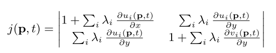
另外, Dupuy [5]等人提出可以利用雅可比行列式来求得每一个顶点的运动撕扯程度. 对于撕扯程度较大的位置更容易产生白沫:

引入 - 完全基于CPU运算的海洋学统计模型实现

对于绝大多数人来说, 看到这么多公式内心都是崩溃的(比方说我), 更别提直接实现出来. 考虑到我们之前说过的, 水面运动模拟要得到的无非是两组数据: 水面网格的几何波动和法线方向. 对于前者, 相当于是一组顶点坐标数据; 对于后者, 相当于是一组向量数据. 想到这里, 我们不妨先在CPU上实现一下海洋学统计模型, 将结果直接写入Attribute中, 再交给显卡渲染. 显然这种做法的效率非常之低, 但是有助于我们理解.

做法的原理很简单: 先生成初始频谱, 然后每一帧根据当前的散布函数计算当前帧频谱, 最后做傅立叶变换即可得到数据. 让我们不要考虑性能, 不要考虑代码质量, 简单粗暴地写一个来验证下想法:

#region MonoBehaviours

private void Update()
{
	timer += Time.deltaTime / tDivision;
	EvaluateWaves(timer);
}

private void Awake()
{
	filter = GetComponent<MeshFilter>();
	mesh = new Mesh();
	filter.mesh = mesh;
	SetParams();
	GenerateMesh();
}

#endregion

private void SetParams()
{
	vertices = new Vector3[resolution * resolution];
	indices = new int[(resolution - 1) * (resolution - 1) * 6];
	normals = new Vector3[resolution * resolution];
	vertConj = new Vector2[resolution * resolution];
	verttilde = new Vector2[resolution * resolution];
	vertMeow = new Vector3[resolution * resolution];//Meow ~ 
	uvs = new Vector2[resolution * resolution];
}

private void GenerateMesh()
{
	int indiceCount = 0;
	int halfResolution = resolution / 2;
	for (int i = 0; i < resolution; i++)
	{
		float horizontalPosition = (i - halfResolution) * unitWidth;
		for (int j = 0; j < resolution; j++)
		{
			int currentIdx = i * (resolution) + j;
			float verticalPosition = (j - halfResolution) * unitWidth;
			vertices[currentIdx] = new Vector3(horizontalPosition + (resolution % 2 == 0? unitWidth / 2f : 0f), 0f, verticalPosition + (resolution % 2 == 0? unitWidth / 2f : 0f));
			normals[currentIdx] = new Vector3(0f, 1f, 0f);
			verttilde[currentIdx] = htilde0(i, j);
			Vector2 temp = htilde0(resolution - i, resolution - j);
			vertConj[currentIdx] = new Vector2(temp.x, -temp.y);
			uvs[currentIdx] = new Vector2(i * 1.0f / (resolution - 1), j * 1.0f / (resolution - 1));
			if (j == resolution - 1)
				continue;
			if (i != resolution - 1)
			{
				indices[indiceCount++] = currentIdx;
				indices[indiceCount++] = currentIdx + 1;
				indices[indiceCount++] = currentIdx + resolution;
			}
			if (i != 0)
			{
				indices[indiceCount++] = currentIdx;
				indices[indiceCount++] = currentIdx - resolution + 1;
				indices[indiceCount++] = currentIdx + 1;
			}
		}
	}
	mesh.vertices = vertices;
	mesh.SetIndices(indices, MeshTopology.Triangles, 0);
	mesh.normals = normals;
	mesh.uv = uvs;
	filter.mesh = mesh;
}

private Vector3 Displacement(Vector2 x, float t, out Vector3 nor)
{
	Vector2 h = new Vector2(0f, 0f);
	Vector2 d = new Vector2(0f, 0f);
	Vector3 n = Vector3.zero;
	Vector2 c, htilde_c, k;
	float kx, kz, k_length, kDotX;
	for (int i = 0; i < resolution; i++)
	{
		kx = 2 * PI * (i - resolution / 2.0f) / length;
		for (int j = 0; j < resolution; j++)
		{
			kz = 2 * PI * (j - resolution / 2.0f) / length;
			k = new Vector2(kx, kz);
			k_length = k.magnitude;
			kDotX = Vector2.Dot(k, x);
			c = new Vector2(Mathf.Cos(kDotX), Mathf.Sin(kDotX));
			Vector2 temp = htilde(t, i, j);
			htilde_c = new Vector2(temp.x * c.x - temp.y * c.y, temp.x * c.y + temp.y * c.x);
			h += htilde_c;
			n += new Vector3(-kx * htilde_c.y, 0f, -kz * htilde_c.y);
			if (k_length < EPSILON)
				continue;
			d += new Vector2(kx / k_length * htilde_c.y, -kz / k_length * htilde_c.y);
		}
	}
	nor = Vector3.Normalize(Vector3.up - n);
	return new Vector3(d.x, h.x, d.y);
}

private void EvaluateWaves(float t)
{
	hds = new Vector2[resolution * resolution];

	for (int i = 0; i < resolution; i++)
	{
		for (int j = 0; j < resolution; j++)
		{
			int index = i * resolution + j;
			vertMeow[index] = vertices[index];
		}
	}
	for (int i = 0; i < resolution; i++)
	{
		for (int j = 0; j < resolution; j++)
		{
			int index = i * resolution + j;
			Vector3 nor = new Vector3(0f, 0f, 0f);
			Vector3 hd = Displacement(new Vector2(vertMeow[index].x, vertMeow[index].z), t, out nor);
			vertMeow[index].y = hd.y;
			vertMeow[index].z = vertices[index].z - hd.z * choppiness;
			vertMeow[index].x = vertices[index].x - hd.x * choppiness;
			normals[index] = nor;
			hds[index] = new Vector2(hd.x, hd.z);
		}
	}

	Color[] colors = new Color[resolution * resolution];

	for (int i = 0; i < resolution; i++)//写得并不正确,
	{
		for (int j = 0; j < resolution; j++)
		{
			int index = i * resolution + j;
			Vector2 dDdx = Vector2.zero;
			Vector2 dDdy = Vector2.zero;
                        if (i != resolution - 1)
			{
				dDdx = 0.5f * (hds[index] - hds[index + resolution]);
			}
			if (j != resolution - 1)
			{
				dDdy = 0.5f * (hds[index] - hds[index + 1]);
			}
			float jacobian = (1 + dDdx.x) * (1 + dDdy.y) - dDdx.y * dDdy.x;
			Vector2 noise = new Vector2(Mathf.Abs(normals[index].x), Mathf.Abs(normals[index].z)) * 0.3f;
			float turb = Mathf.Max(1f - jacobian + noise.magnitude, 0f);
			float xx = 1f + 3f * Mathf.SmoothStep(1.2f, 1.8f, turb);
			xx = Mathf.Min(turb, 1.0f);
			xx = Mathf.SmoothStep(0f, 1f, turb);
			colors[index] = new Color(xx, xx, xx, xx);
		}
	}
	mesh.vertices = vertMeow;
	mesh.normals = normals;
	mesh.colors = colors;
}

以上代码完全没有经过任何优化, 甚至连DFT都使用了暴力方式进行求解, 相当于把公式直白地翻译了一遍(换句话说, 这要是还看不懂就可以 ... 额). 这段代码运行起来, 在我的i7-7700HQ上可以支持高达18*18的水面(笑, 再大一点就跑不满60FPS了):

关于统计学模型在CPU上的实现, 这篇博客写得不错 [6]. 虽然里面有些公式用错了, 但是有很大的参考价值.

嗯, 看起来我们的理论没有问题. 那么现在要做的就是给暴力的运算提提速, 搬个家!

进化 - GPU上的FFT, 随机数与Implementation Notes

说到FFT, 我们马上就能想到的是Cooley-Tukey [6]的蝶形变换, 能将n方级别的DIT优化到nlogn级别. Cooley-Tukey的FFT求解方式是可以放到GPU上实现的, 但是基于GPU的FFT中有一种叫Stockham Formulation [7]的做法. 下图是两个做法的比较:

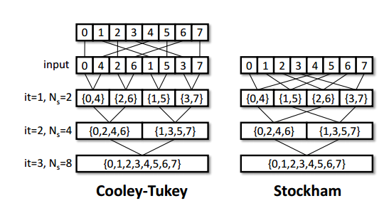
如今很多GPU上的FFT实现方式都是基于Stockham FFT的, 比如GLFFT. 关于各种FFT求解方式的横向比较可以参考这里 [8].

Stockham FFT的伪代码如下:

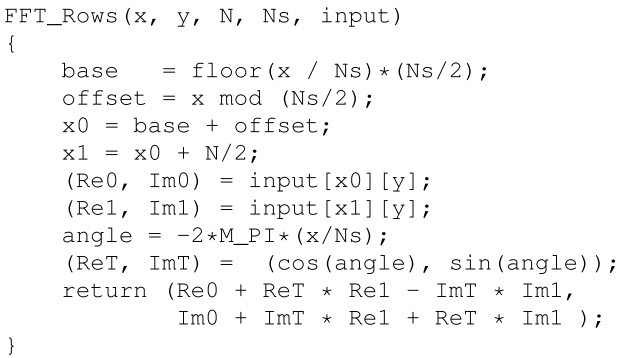
我的实现中把横向和纵向写到了一起, 通过Shader开关来控制. 代码如下:

Shader "Hidden/Mistral Water/Helper/Vertex/Stockham"
{
	Properties
	{
		_Input ("Input Sampler", 2D) = "black" {}
		_TransformSize ("Transform Size", Float) = 256
		_SubTransformSize ("Log Size", Float) = 8
	}

	SubShader
	{
		Pass
		{
			Cull Off
			ZWrite Off
			ZTest Off
			ColorMask RGBA

			CGPROGRAM

			#include "FFTCommon.cginc"

			#pragma vertex vert_quad
			#pragma fragment frag
			#pragma multi_compile _HORIZONTAL _VERTICAL

			uniform sampler2D _Input;
			uniform float _TransformSize;
			uniform float _SubTransformSize;

			float4 frag(FFTVertexOutput i) : SV_TARGET
			{
				float index;

				#ifdef _HORIZONTAL
					index = i.texcoord.x * _TransformSize - 0.5;
				#else
					index = i.texcoord.y * _TransformSize - 0.5;
				#endif

				float evenIndex = floor(index / _SubTransformSize) * (_SubTransformSize * 0.5) + fmod(index, _SubTransformSize * 0.5) + 0.5;

				#ifdef _HORIZONTAL
					float4 even = tex2D(_Input, float2((evenIndex), i.texcoord.y * _TransformSize) / _TransformSize);
					float4 odd  = tex2D(_Input, float2((evenIndex + _TransformSize * 0.5), i.texcoord.y * _TransformSize) / _TransformSize);
				#else
					float4 even = tex2D(_Input, float2(i.texcoord.x * _TransformSize, (evenIndex)) / _TransformSize);
					float4 odd  = tex2D(_Input, float2(i.texcoord.x * _TransformSize, (evenIndex + _TransformSize * 0.5)) / _TransformSize);
				#endif

				float twiddleV = GetTwiddle(index / _SubTransformSize);
				float2 twiddle = float2(cos(twiddleV), sin(twiddleV));
				float2 outputA = even.xy + MultComplex(twiddle, odd.xy);
				float2 outputB = even.zw + MultComplex(twiddle, odd.zw);

				return float4(outputA, outputB);
			}

			ENDCG
		}
	}
}

// FFTCommon.cginc
//inline float GetTwiddle(float ratio)
//{
//	return -2 * PI * ratio;
//}

对于二维FFT, 只需要横向变换后再纵向变换即可.

找到了FFT的解决方案后, 我们仍然需要选用一个PRNG [9]来生成随机数. 理想的情况是CPU在每一帧提供随机的种子, PRNG则会生成前后无关的随机数. 这里我选用的是烟雾模拟中的随机数生成算法:

inline float UVRandom(float2 uv, float salt, float random)
{
	uv += float2(salt, random);
	return frac(sin(dot(uv, float2(12.9898, 78.233))) * 43758.5453);
}

获得了0-1之间随机分布的随机数后, 我们需要修改其分布方式来. 我这里使用的是Box-Muller [10]变换法来获得正态分布的随机数:

inline float2 hTilde0(float2 uv, float r1, float r2, float phi)
{
	float2 r;
	float rand1 = UVRandom(uv, 10.612, r1);
	float rand2 = UVRandom(uv, 11.899, r2);
	rand1 = clamp(rand1, EPSILON, 1);
	rand2 = clamp(rand2, EPSILON, 1);
	float x = sqrt(-2 * log(rand1));
	float y = 2 * PI * rand2;
	r.x = x * cos(y);
	r.y = x * sin(y);
	return r * sqrt(phi / 2); 
}

解决掉所有的数学问题后, 我们不能像刚刚在CPU上实现的那样简单粗暴 --- 这次要好好地设计一下. 我们注意到如果在水面渲染过程中修改风向或是波长的话, 将会导致Dispersion发生骤变, 水面也会产生抖动和闪烁. 因此我们将交替使用两张Dispersion Texture来保证在修改参数前后的连续性.

搬家 - 基于GPU的海洋学统计模型实现

首先来看看整体逻辑:

/// Called in Start
private void RenderInitial()
{
	Graphics.Blit(null, initialTexture, initialMat);
	spectrumMat.SetTexture("_Initial", initialTexture);
	heightMat.SetTexture("_Initial", initialTexture);
}

/// Called in Update
private void GenerateTexture()
{
	float deltaTime = Time.deltaTime;
        //使用两张RT确保参数修改前后连续
	currentPhase = !currentPhase;
	RenderTexture rt = currentPhase ? pingPhaseTexture : pongPhaseTexture;
	dispersionMat.SetTexture("_Phase", currentPhase? pongPhaseTexture : pingPhaseTexture);
	dispersionMat.SetFloat("_DeltaTime", deltaTime * mult);
	Graphics.Blit(null, rt, dispersionMat);

	spectrumMat.SetTexture("_Phase", currentPhase? pingPhaseTexture : pongPhaseTexture);
	Graphics.Blit(null, spectrumTexture, spectrumMat);

	fftMat.EnableKeyword("_HORIZONTAL");
	fftMat.DisableKeyword("_VERTICAL");
	int iterations = Mathf.CeilToInt((float)Math.Log(resolution * 8, 2)) * 2;
	for (int i = 0; i < iterations; i++)
	{
		fftMat.SetFloat("_SubTransformSize", Mathf.Pow(2, (i % (iterations / 2)) + 1));
		if (i == 0)
		{
			fftMat.SetTexture("_Input", spectrumTexture);
			Graphics.Blit(null, pingTransformTexture, fftMat);
		}
		else if (i == iterations - 1)
		{
			fftMat.SetTexture("_Input", (iterations % 2 == 0) ? pingTransformTexture : pongTransformTexture);
			Graphics.Blit(null, displacementTexture, fftMat);
		}
		else if (i % 2 == 1)
		{
			fftMat.SetTexture("_Input", pingTransformTexture);
			Graphics.Blit(null, pongTransformTexture, fftMat);
		}
		else
		{
			fftMat.SetTexture("_Input", pongTransformTexture);
			Graphics.Blit(null, pingTransformTexture, fftMat);
		}
		if (i == iterations / 2 - 1)
		{
			fftMat.DisableKeyword("_HORIZONTAL");
			fftMat.EnableKeyword("_VERTICAL");
		}
	}

	heightMat.SetTexture("_Phase", currentPhase? pingPhaseTexture : pongPhaseTexture);
	Graphics.Blit(null, spectrumTexture, heightMat);
	fftMat.EnableKeyword("_HORIZONTAL");
	fftMat.DisableKeyword("_VERTICAL");
	for (int i = 0; i < iterations; i++)
	{
		fftMat.SetFloat("_SubTransformSize", Mathf.Pow(2, (i % (iterations / 2)) + 1));
		if (i == 0)
		{
			fftMat.SetTexture("_Input", spectrumTexture);
			Graphics.Blit(null, pingTransformTexture, fftMat);
		}
		else if (i == iterations - 1)
		{
			fftMat.SetTexture("_Input", (iterations % 2 == 0) ? pingTransformTexture : pongTransformTexture);
			Graphics.Blit(null, heightTexture, fftMat);
		}
		else if (i % 2 == 1)
		{
			fftMat.SetTexture("_Input", pingTransformTexture);
			Graphics.Blit(null, pongTransformTexture, fftMat);
		}
		else
		{
			fftMat.SetTexture("_Input", pongTransformTexture);
			Graphics.Blit(null, pingTransformTexture, fftMat);
		}
		if (i == iterations / 2 - 1)
		{
			fftMat.DisableKeyword("_HORIZONTAL");
			fftMat.EnableKeyword("_VERTICAL");
		}
	}

	Graphics.Blit(null, normalTexture, normalMat);
	Graphics.Blit(null, whiteTexture, whiteMat);
}

InitialMat 对应的初始频谱Shader:

Shader "Hidden/Mistral Water/Helper/Vertex/Initial Spectrum"
{
	Properties
	{
		_RandomSeed1 ("Random Seed 1", Float) = 1.5122
		_RandomSeed2 ("Random Seed 2", Float) = 6.1152
		_Amplitude ("Phillips Ampitude", Float) = 1
		_Length ("Wave Length", Float) = 256
		_Resolution ("Ocean Resolution", int) = 256
		_Wind ("Wind Direction (XY)", Vector) = (1, 1, 0, 0)
	}

	SubShader
	{
		Pass
		{
			Cull Off
			ZWrite Off
			ZTest Off
			ColorMask RGBA

			CGPROGRAM

			#include "FFTCommon.cginc"

			#pragma vertex vert_quad
			#pragma fragment frag

			uniform float _RandomSeed1;
			uniform float _RandomSeed2;
			uniform float _Amplitude;
			uniform float _Length;
			uniform int _Resolution;
			uniform float2 _Wind;

			float4 frag(FFTVertexOutput i) : SV_TARGET
			{
				float n = (i.texcoord.x * _Resolution);
				float m = (i.texcoord.y * _Resolution);

				float phi1 = Phillips(n, m, _Amplitude, _Wind, _Resolution, _Length);
				float phi2 = Phillips(_Resolution - n, _Resolution - m, _Amplitude, _Wind, _Resolution, _Length);

				float2 h0 = hTilde0(i.texcoord.xy, _RandomSeed1 / 2, _RandomSeed2 * 2, phi1);
				float2 h0conj = Conj(hTilde0(i.texcoord.xy, _RandomSeed1, _RandomSeed2, phi2));

				return float4(h0, h0conj);
			}

			ENDCG
		}
	}
}

/// FFTCommon.cginc
//inline float Phillips(float n, float m, float amp, float2 wind, float res, float len)
//{
//	float2 k = GetWave(n, m, len, res);
//	float klen = length(k);
//	float klen2 = klen * klen;
//	float klen4 = klen2 * klen2;
//	if(klen < EPSILON)
//		return 0;
//	float kDotW = dot(normalize(k), normalize(wind));
//	float kDotW2 = kDotW * kDotW;
//	float wlen = length(wind);
//	float l = wlen * wlen / G;
//	float l2 = l * l;
//	float damping = 0.01;
//	float L2 = l2 * damping * damping;
//	return amp * exp(-1 / (klen2 * l2)) / klen4 * kDotW2 * exp(-klen2 * L2);
//}

//inline float2 hTilde0(float2 uv, float r1, float r2, float phi)
//{
//	float2 r;
//	float rand1 = UVRandom(uv, 10.612, r1);
//	float rand2 = UVRandom(uv, 11.899, r2);
//	rand1 = clamp(rand1, 0.01, 1);
//	rand2 = clamp(rand2, 0.01, 1);
//	float x = sqrt(-2 * log(rand1));
//	float y = 2 * PI * rand2;
//	r.x = x * cos(y);
//	r.y = x * sin(y);
//	return r * sqrt(phi / 2); 
//}

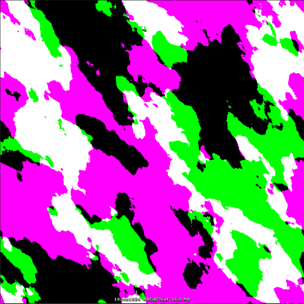
得到的初始h0与其共轭复数如下:

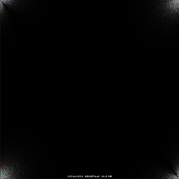
PhaseMat对应的Shader:

Shader "Hidden/Mistral Water/Helper/Vertex/Dispersion"
{
	Properties
	{
		_Length ("Wave Length", Float) = 256
		_Resolution ("Ocean Resolution", int) = 256
		_DeltaTime ("Delta Time", Float) = 0.016
		_Phase ("Last Phase", 2D) = "black" {}
	}

	SubShader
	{
		Pass
		{
			Cull Off
			ZWrite Off
			ZTest Off
			ColorMask R

			CGPROGRAM

			#include "FFTCommon.cginc"

			#pragma vertex vert_quad
			#pragma fragment frag

			uniform float _DeltaTime;
			uniform float _Length;
			uniform int _Resolution;
			uniform sampler2D _Phase;

			float4 frag(FFTVertexOutput i) : SV_TARGET
			{
				float n = (i.texcoord.x * _Resolution);
				float m = (i.texcoord.y * _Resolution);

				float deltaPhase = CalcDispersion(n, m, _Length, _DeltaTime, _Resolution);
				float phase = tex2D(_Phase, i.texcoord).r;

				return float4(GetDispersion(phase, deltaPhase), 0, 0, 0);
			}

			ENDCG
		}
	}
}
/// FFTCommon.cginc
//inline float GetDispersion(float oldPhase, float newPhase)
//{
//	return fmod(oldPhase + newPhase, 2 * PI);
//}

//inline float CalcDispersion(float n, float m, float len, float dt, float res)
//{
//	float2 wave = GetWave(n, m, len, res);
//	float w = 2 * PI / len;
//	float wlen = length(wave);
//	return sqrt(G * length(wave) * (1 + wlen * wlen / 370 / 370)) * dt;
//	//return floor(sqrt(G * length(wave) / w)) * w * dt;
//}

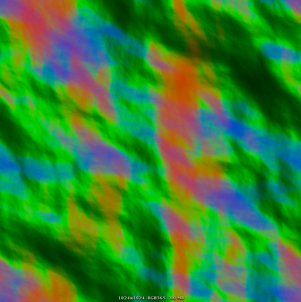
结果如下:

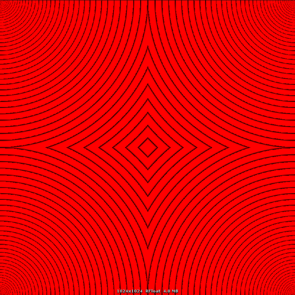
spectrumMat对应的Shader(与HeightMat对应的很类似. HeightMat直接返回了h):

Shader "Hidden/Mistral Water/Helper/Vertex/Spectrum"
{
	Properties
	{
		_Length ("Wave Length", Float) = 256
		_Resolution ("Ocean Resolution", int) = 256
		_Phase ("Last Phase", 2D) = "black" {}
		_Initial ("Intial Spectrum", 2D) = "black" {}
		_Choppiness ("Choppiness", Float) = 1
	}

	SubShader
	{
		Pass
		{
			Cull Off
			ZWrite Off
			ZTest Off
			ColorMask RGBA

			CGPROGRAM

			#include "FFTCommon.cginc"

			#pragma vertex vert_quad
			#pragma fragment frag

			uniform sampler2D _Phase;
			uniform sampler2D _Initial;
			uniform float _Length;
			uniform int _Resolution;
			uniform float _Choppiness;

			float4 frag(FFTVertexOutput i) : SV_TARGET
			{
				float n = (i.texcoord.x * _Resolution);
				float m = (i.texcoord.y * _Resolution);
				float2 wave = GetWave(n, m, _Length, _Resolution);
				float w = length(wave);
				float phase = tex2D(_Phase, i.texcoord).r;
				float2 pv = float2(cos(phase), sin(phase));
				float2 h0 = tex2D(_Initial, i.texcoord).rg;
				float2 h0conj = tex2D(_Initial, i.texcoord).ba;
				//h0conj = MultByI(h0conj);
				float2 h = MultComplex(h0, pv) + MultComplex(h0conj, Conj(pv));
				//return float4(h, h);
				w = max(0.0001, w);
				float2 hx = -MultByI(h * wave.x / w) * _Choppiness;
				float2 hz = -MultByI(h * wave.y / w) * _Choppiness;
				return float4(hx, hz);
			}

			ENDCG
		}
	}
}

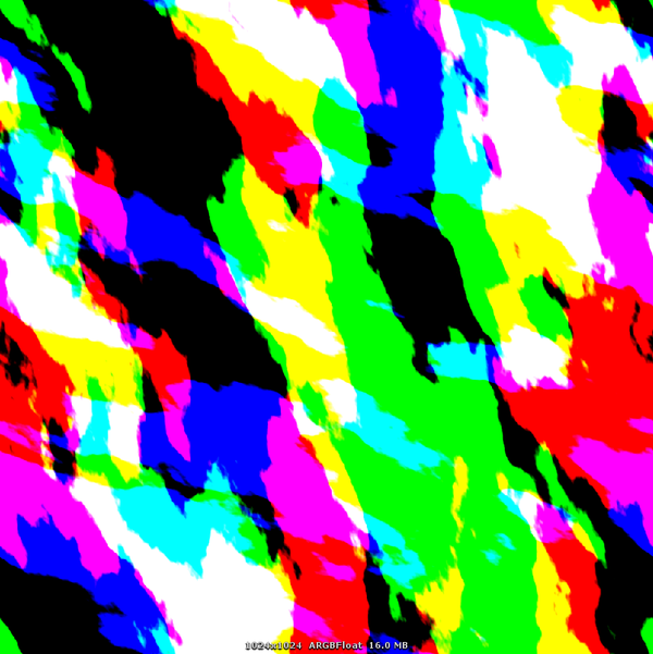
最后得到的高度贴图和水平扰动如下(我这里数值的绝对值是0-8, 所以看起来"过曝"):

法线贴图直接通过采样扰动贴图计算即可:

whiteMat对应的白沫检测Shader如下:

Shader "Hidden/Mistral Water/Helper/Map/Ocean Normal"
{
	Properties
	{
		_Resolution ("Resolution", Float) = 512
		_Length ("Sea Width", Float) = 512
		_Displacement ("Displacement", 2D) = "black" {}
		_Bump ("_Bump", 2D) = "bump" {}
	}

	SubShader
	{
		Pass
		{
			Cull Off
			ZWrite Off
			ZTest Off
			ColorMask R

			CGPROGRAM

			#include "FFTCommon.cginc"

			#pragma vertex vert_quad
			#pragma fragment frag

			uniform float _Resolution;
			uniform float _Length;
			uniform sampler2D _Displacement;
			uniform float4 _Displacement_TexelSize;
			uniform sampler2D _Bump;

			float4 frag(FFTVertexOutput i) : SV_TARGET
			{
				float texelSize = 1 / _Length;
				float2 dDdy = -0.5 * (tex2D(_Displacement, i.texcoord + float4(0, -texelSize, 0, 0)).rb - tex2D(_Displacement, i.texcoord + float4(0, texelSize, 0, 0)).rb) / 8;
				float2 dDdx = -0.5 * (tex2D(_Displacement, i.texcoord + float4(-texelSize, 0, 0, 0)).rb - tex2D(_Displacement, i.texcoord + float4(texelSize, 0, 0, 0)).rb) / 8;
				float2 noise = 0.3 * tex2D(_Bump, i.texcoord).xz;
				float jacobian = (1 + dDdx.x) * (1 + dDdy.y) - dDdx.y * dDdy.x;
				float turb = max(0, 1 - jacobian + length(noise));
				float xx = 1 + 3 * smoothstep(1.2, 1.8, turb);
				xx = min(turb, 1);
				xx = smoothstep(0, 1, turb);
				return float4(xx, xx, xx, 1);
			}

			ENDCG
		}
	}
}

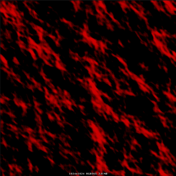
白沫贴图:

后记

到此, 一个最基本的水面模拟就已经实现出来了. 在专栏今后的2-3期中我将介绍水面的物理真实渲染和风格化渲染, 以及针对特殊的运动方式进一步介绍水面运动模拟.

因为渲染还没有完全搞定, 因此代码还没有丢到GitHub上. 下一期更新的时候我会把链接放上来.

References

[1] GPU Gems

[2]Trochoidal wave - Wikipedia

[3]Ocean Shader with Gerstner Waves

[4]Tessendorf, Jerry. "Simulating ocean water." Simulating nature: realistic and interactive techniques. SIGGRAPH 1.2 (2001): 5.

[5]Dupuy, Jonathan, and Eric Bruneton. "Real-time animation and rendering of ocean whitecaps." SIGGRAPH Asia 2012 Technical Briefs. ACM, 2012.

[6] Cooley, James W., and John W. Tukey. "An algorithm for the machine calculation of complex Fourier series." Mathematics of computation 19.90 (1965): 297-301.

[7]Lloyd, D. Brandon, Chas Boyd, and Naga Govindaraju. "Fast computation of general Fourier transforms on GPUs." Multimedia and Expo, 2008 IEEE International Conference on. IEEE, 2008.

[8] http://users.ece.cmu.edu/~franzf/papers/fft-enc11.pdf

[9] Pseudorandom number generator. (2017, December 18). In Wikipedia, The Free Encyclopedia. Retrieved 13:38, December 29, 2017, from https://en.wikipedia.org/w/index.php?title=Pseudorandom_number_generator&amp;amp;amp;amp;amp;oldid=816057825

[10]Box-Muller transform

编辑于 2017-12-30 01:30