自然语言分析加关系网络 - 半自动分析倚天屠龙记

关键词: Word2vec, Networkx, Jieba, 自然语言, 向量话,相似,关系网络,倚天屠龙记
最近在了解到,在机器学习中,自然语言处理是较大的一个分支。存在许多挑战。例如: 如何分词,识别实体关系,实体间关系,关系网络展示等。
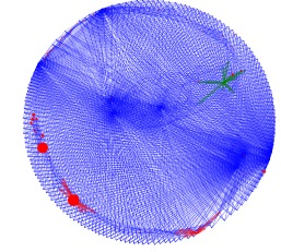
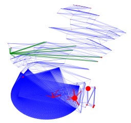
我用Jieba + Word2vec + NetworkX 结合在一起,做了一次自然语言分析。语料是 倚天屠龙记。 之前也有很多人用金庸的武侠小说做分析和处理,希望带来一些不同的地方。截几张图来看看:
这次分析的不一样之处主要是:
1. Word2Vec的相似度结果 - 作为后期社交网络权重
2 . NetworkX中分析和展示
上面两个方法结合起来,可以大幅减少日常工作中阅读文章的时间。 采用机器学习,可以从头到尾半自动抽取文章中的实体信息,节约大量时间和成本。 在各种工作中都有利用的场景, 如果感兴趣的朋友,可以联系合作。
先来看看,用Word2Vec+NetworkX 可以发现什么。
一 .分析结果
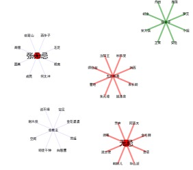
实体的不同属性(张无忌的总多马甲)
张无忌,无忌,张教主,无忌哥哥,张公子。同一个张无忌有多个身份,不同身份又和不同的人联系,有不一样的相似度。
先来看看图:
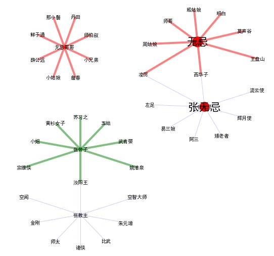

无忌哥哥是过于亲密的名字,一般不喊。好似和这个词相似度高的都是比较奇怪的角色。
无忌是关系熟了以后,平辈或者长辈可以称呼的名字。还有周姑娘,殷姑娘等
张无忌是通用的名字,人人可以称呼 和马甲联系密切。
张公子是礼貌尊称。 例如,黄衫女子,汝阳王等
张教主是头衔。既要尊重,也表示其实不太熟,有时还有些敌意。 例如: 朱元璋
注:
- 图是Networkx 基于Word2vex画出来了,上面的描述是我的人工分析。
- 赵敏不在上面的网络关系图中。Word2Vec计算出来 张无忌和赵敏 相似度不太高。有些出乎我的意料。 仔细回忆一下,当年看此书时,突然就发现二人在一起了,显得比较突兀。推想起来,书中世界二人成婚了,如果变成现实世界,二人关系比较悬。
二。 实现过程
主要步骤:
- 准备语料,
- 倚天屠龙记 小说的文本文件
- 自定义分词词典 (小说中的人物名,网上有现成的,约180个)
- 停用词表
- 准备工具
- Python Pandas, Numpy,Scipy(标准库)
- Jieba(中文分词)
- Word2vec (单词向量化工具,可以计算单词之间的详细度)
- Networks(网络图工具,用于展示复杂的网络关系
- 数据预处理
- 文本文件转发成utf8(pandas)
- 文本文件分句,分词(Jieba)
- 文本文件分句,分词, 分析词性,主要是人名(Jieba)
- 更新自定义词典,重新分词(整个过程需要几遍,直至满意)
- 手工少量删除(分词出来的人名误判率不高,但是还是存在一些。例如:赵敏笑道,可以被识别的 一个叫 赵敏笑的人。 这部分工作还需要手工做。 除非有更好的分词工具,或者可以训练的分词工具,才能解决这一问题。
- Word2Vec 训练模型。这个模型可以计算两个人之间的相似度
- 采用300个维度
- 过滤词频小于20次
- 滑动窗口 为20
- 下采样:0.001
- 生成实体关系矩阵。
- 网上没找找到现成库,我就自己写了一个。
- N*N 维度。 N是人名数量。
- 用上面WordVec的模型来,填充实体关系矩阵
- NetworkX 生成网络图
- 节点是人名
- 边是两个节点之间的线条。也就是两个人之间的关系。
实现代码(未优化和未整理版本)
初始化
import numpy as np
import pandas as pd
import jieba
import jieba.posseg as posseg
%matplotlib inline
数据分词,清洗
renming_file = "yttlj_renming.csv"
jieba.load_userdict(renming_file)
stop_words_file = "stopwordshagongdakuozhan.txt"
stop_words = pd.read_csv(stop_words_file,header=None,quoting=3,sep="\t")[0].values
corpus = "yttlj.txt"
yttlj = pd.read_csv(corpus,encoding="gb18030",header=None,names=["sentence"])


def cut_join(s):
    new_s=list(jieba.cut(s,cut_all=False)) #分词
    #print(list(new_s))
    stop_words_extra =set([""])


    for seg in new_s:

        if len(seg)==1:
            #print("aa",seg)
            stop_words_extra.add(seg)

    #print(stop_words_extra)
    #print(len(set(stop_words)| stop_words_extra))

    new_s =set(new_s) -set(stop_words)-stop_words_extra
    #过滤标点符号
    #过滤停用词
    result = ",".join(new_s)

    return  result

def extract_name(s):
    new_s=posseg.cut(s) #取词性
    words=[]
    flags=[]
    for k,v in new_s:
        if len(k)>1:
            words.append(k)
            flags.append(v)
    full_wf["word"].extend(words)
    full_wf["flag"].extend(flags)
    return len(words)

def check_nshow(x):
    nshow = yttlj["sentence"].str.count(x).sum()
    #print(x, nshow)
    return nshow

# extract name & filter times

full_wf={"word":[],"flag":[]}
possible_name = yttlj["sentence"].apply(extract_name)
#tmp_w,tmp_f

df_wf = pd.DataFrame(full_wf)

df_wf_renming = df_wf[(df_wf.flag=="nr")].drop_duplicates()
df_wf_renming.to_csv("tmp_renming.csv",index=False)

df_wf_renming = pd.read_csv("tmp_renming.csv")
df_wf_renming.head()


df_wf_renming["nshow"] = df_wf_renming.word.apply(check_nshow)

df_wf_renming[df_wf_renming.nshow>20].to_csv("tmp_filtered_renming.csv",index=False)

df_wf_renming[df_wf_renming.nshow>20].shape

#手工编辑,删除少量非人名,分词错的人名
df_wf_renming=pd.read_csv("tmp_filtered_renming.csv")
my_renming = df_wf_renming.word.tolist()


external_renming = pd.read_csv(renming_file,header=None)[0].tolist()


combined_renming = set(my_renming) |set(external_renming)
pd.DataFrame(list(combined_renming)).to_csv("combined_renming.csv",header=None,index=False)


combined_renming_file ="combined_renming.csv"
jieba.load_userdict(combined_renming_file)


# tokening

yttlj["token"]=yttlj["sentence"].apply(cut_join)

yttlj["token"].to_csv("tmp_yttlj.csv",header=False,index=False)
sentences = yttlj["token"].str.split(",").tolist()
Word2Vec 向量化训练
# Set values for various parameters
num_features = 300    # Word vector dimensionality
min_word_count = 20   # Minimum word count
num_workers = 4       # Number of threads to run in parallel
context = 20          # Context window size
downsampling = 1e-3   # Downsample setting for frequent words

# Initialize and train the model (this will take some time)

from gensim.models import word2vec

model_file_name = 'yttlj_model.txt'
#sentences = w2v.LineSentence('cut_jttlj.csv')


model = word2vec.Word2Vec(sentences, workers=num_workers, \
            size=num_features, min_count = min_word_count, \
            window = context, \
            sample = downsampling
            )


model.save(model_file_name)
建立实体关系矩阵
entity = pd.read_csv(combined_renming_file,header=None,index_col=None)
entity = entity.rename(columns={0:"Name"})
entity = entity.set_index(["Name"],drop=False)

ER = pd.DataFrame(np.zeros((entity.shape[0],entity.shape[0]),dtype=np.float32),index=entity["Name"],columns=entity["Name"])
ER["tmp"] = entity.Name

def check_nshow(x):
    nshow = yttlj["sentence"].str.count(x).sum()
    #print(x, nshow)
    return nshow

ER["nshow"]=ER["tmp"].apply(check_nshow)
ER = ER.drop(["tmp"],axis=1)

count = 0
for i in entity["Name"].tolist():
    count +=1
    if count % round(entity.shape[0]/10) ==0:
        print("{0:.1f}% relationship has been checked".format(100*count/entity.shape[0]))
    elif count == entity.shape[0]:
        print("{0:.1f}% relationship has been checked".format(100*count/entity.shape[0]))

    for j in entity["Name"]:
        relation =0
        try:
            relation = model.wv.similarity(i,j)
            ER.loc[i,j] = relation
            if i!=j:
                ER.loc[j,i] = relation
        except:
            relation = 0


ER.to_hdf("ER.h5","ER")
NetworkX 展示人物关系图
import networkx as nx
import matplotlib.pyplot as plt
import pandas as pd
import numpy as np
import pygraphviz
from networkx.drawing.nx_agraph import graphviz_layout
此处为提取张无忌的不同属性的关系和相似性
def fill_node(G,ER,topn=0.1,nearn=5,index_filter=[]):
    color_ER ={"张无忌":"b",
               "张教主":"b",
               "无忌哥哥":"r",
               "张公子":"g",
               "无忌":"r"}
    color_ER.setdefault("b")

    if len(index_filter) ==0:
        mask = ER.nshow>ER.nshow.quantile(1-topn)
        ER_highshow = ER[mask]
        maxshow = ER_highshow.nshow.max()
        indexes = ER_highshow.index

    else:
        maxshow = ER.nshow.max()
        ER_highshow = ER
        indexes = index_filter

    for index in indexes:
        #print(index)
        size = (ER_highshow.loc[index,"nshow"] )

        G.add_node(index,weight=size)
        #print(index,size)
        importance = size
        #print(iters)

        small_columns = ER_highshow.loc[index,:].sort_values().tail(nearn).index
        for col in small_columns:
            if col !="nshow":
                relation = ER_highshow.loc[index,col]
                if relation >0:
                    check_index = index in ["张无忌","张教主","无忌哥哥","无忌","张公子"]
                    check_col = col in ["张无忌","张教主","无忌哥哥","无忌","张公子"]
                    if check_index or check_col:
                        if check_index:
                            label = color_ER[index]
                        else:
                            label = color_ER[col]
                    else:
                        label="b"
                G.add_edge(index,col,weight= relation,lable=label)
    return

def scaler_degree(top=20):
    node =[v.setdefault("weight",0) for k,v in G.node.items()]

    from sklearn.preprocessing import minmax_scale
    scaled_degree = np.round(minmax_scale(node,(0,top))**2)
    return scaled_degree.tolist()

def filter_nodes(counter=50):
    Nodes = G.node
    filtered_nodes={}
    for k,v in Nodes.items():
        value = v.setdefault("weight",0)
        if value> counter:
            filtered_nodes[k]=k
        else:
            filtered_nodes[k]=""
    #print(filtered_nodes)
    return filtered_nodes
展示
plt.subplots(figsize=(10,10))

ER = pd.read_hdf("ER.h5","ER")
G=nx.Graph()

fill_node(G,ER,nearn=10,index_filter=["张无忌","无忌","无忌哥哥","张教主","张公子"])
d = nx.degree(G)

pos = graphviz_layout(G, prog='twopi', args='')


elarge=[(u,v) for (u,v,d) in G.edges(data=True) if d['weight'] >0.99999]
esmall=[(u,v) for (u,v,d) in G.edges(data=True) if d['weight'] <=0.96]
edge_red=[(u,v) for (u,v,d) in G.edges(data=True) if d['lable'] =="r"]
edge_green=[(u,v) for (u,v,d) in G.edges(data=True) if d['lable'] =="g"]
edge_blue=[(u,v) for (u,v,d) in G.edges(data=True) if d['lable'] =="b"]


# nodes
nx.draw_networkx_nodes(G,pos,node_size=scaler_degree()
                      )

# edges
nx.draw_networkx_edges(G,pos,edgelist=elarge,
                    width=1,alpha=0.2,edge_color='b',style='dashed')
nx.draw_networkx_edges(G,pos,edgelist=esmall,
                    width=1,alpha=0.2,edge_color='b',style='dashed')

nx.draw_networkx_edges(G,pos,edgelist=edge_blue,
                    width=1,alpha=0.2,edge_color='b')
nx.draw_networkx_edges(G,pos,edgelist=edge_green,
                    width=4,alpha=0.5,edge_color='g',)

nx.draw_networkx_edges(G,pos,edgelist=edge_red,
                    width=4,alpha=0.5,edge_color='r',)


nx.draw_networkx_labels(G,pos,
                        font_size= 10,font_family='sans-serif')


nx.draw_networkx_labels(G,pos,labels=filter_nodes(1000),
                        font_size= 22,font_family='sans-serif')


# labels标签定义

plt.axis("off")

plt.show() # display
主动分享吧,这将是生活工作中最好的投资!
王勇
2018年3月17日
招揽机器学习和自然语言落地业务,欢迎联系。