Arrays.sort()排序原理

原文地址:Arrays.sort()排序原理
java.util.Arrays有针对各种数据类型的重载的sort的方法,下面我们主要介绍其中的两种(Arrays.sort(整数数组))
在继续讲解之前我们先来看这种排序方法的整体组成,对这个方法现有一个大概的了解

使用Arrays.sort对int数组进行排序时,Arrays.sort方法会调用DualPivotQuicksort.sort方法
/**
     * Sorts the specified array into ascending numerical order.
     *
     * <p>Implementation note: The sorting algorithm is a Dual-Pivot Quicksort
     * by Vladimir Yaroslavskiy, Jon Bentley, and Joshua Bloch. This algorithm
     * offers O(n log(n)) performance on many data sets that cause other
     * quicksorts to degrade to quadratic performance, and is typically
     * faster than traditional (one-pivot) Quicksort implementations.
     *
     * @param a the array to be sorted
     */
    public static void sort(int[] a) {
        DualPivotQuicksort.sort(a, 0, a.length - 1, null, 0, 0);
    }
DualPivotQuicksort中实现了所有基本数据类型的排序方法
/**
     * Sorts the specified range of the array using the given
     * workspace array slice if possible for merging
     *
     * @param a the array to be sorted
     * @param left the index of the first element, inclusive, to be sorted
     * @param right the index of the last element, inclusive, to be sorted
     * @param work a workspace array (slice)
     * @param workBase origin of usable space in work array
     * @param workLen usable size of work array
     */
    static void sort(int[] a, int left, int right,
                     int[] work, int workBase, int workLen) {
        // Use Quicksort on small arrays   使用快速排序对小数组排序
        if (right - left < QUICKSORT_THRESHOLD) {
            sort(a, left, right, true);
            return;
        }

        /*
         * 评估数组的无序程度
         * Index run[i] is the start of i-th run
         * (ascending or descending sequence).
         */
        int[] run = new int[MAX_RUN_COUNT + 1];
        int count = 0; run[0] = left;

        // Check if the array is nearly sorted
        for (int k = left; k < right; run[count] = k) {
            if (a[k] < a[k + 1]) { // ascending 递增子序列
                while (++k <= right && a[k - 1] <= a[k]);
            } else if (a[k] > a[k + 1]) { // descending 递减子序列
                while (++k <= right && a[k - 1] >= a[k]);
                for (int lo = run[count] - 1, hi = k; ++lo < --hi; ) {
                    int t = a[lo]; a[lo] = a[hi]; a[hi] = t;
                }
            } else { // equal
                for (int m = MAX_RUN_LENGTH; ++k <= right && a[k - 1] == a[k]; ) {
                    if (--m == 0) {
                        sort(a, left, right, true);
                        return;
                    }
                }
            }

            /*
             * The array is not highly structured,    如果数组基本无序
             * use Quicksort instead of merge sort.   用快速排序代替归并排序
             */
            if (++count == MAX_RUN_COUNT) {
                sort(a, left, right, true);
                return;
            }
        }

        // Check special cases     给run数组的末尾添加了一个“哨兵”元素
        // Implementation note: variable "right" is increased by 1.
        if (run[count] == right++) { // The last run contains one element
            run[++count] = right;
        } else if (count == 1) { // The array is already sorted
            return;
        }

        // Determine alternation base for merge    归并排序
        byte odd = 0;
        for (int n = 1; (n <<= 1) < count; odd ^= 1);

        // Use or create temporary array b for merging
        int[] b;                 // temp array; alternates with a
        int ao, bo;              // array offsets from 'left'
        int blen = right - left; // space needed for b
        if (work == null || workLen < blen || workBase + blen > work.length) {
            work = new int[blen];
            workBase = 0;
        }
        if (odd == 0) {
            System.arraycopy(a, left, work, workBase, blen);
            b = a;
            bo = 0;
            a = work;
            ao = workBase - left;
        } else {
            b = work;
            ao = 0;
            bo = workBase - left;
        }

        // Merging
        for (int last; count > 1; count = last) {
            for (int k = (last = 0) + 2; k <= count; k += 2) {
                int hi = run[k], mi = run[k - 1];
                for (int i = run[k - 2], p = i, q = mi; i < hi; ++i) {
                    if (q >= hi || p < mi && a[p + ao] <= a[q + ao]) {
                        b[i + bo] = a[p++ + ao];
                    } else {
                        b[i + bo] = a[q++ + ao];
                    }
                }
                run[++last] = hi;
            }
            if ((count & 1) != 0) {
                for (int i = right, lo = run[count - 1]; --i >= lo;
                    b[i + bo] = a[i + ao]
                );
                run[++last] = right;
            }
            int[] t = a; a = b; b = t;
            int o = ao; ao = bo; bo = o;
        }
    }
以上方法,针对不同的数据量使用不同的排序方法进行排序。总共用到了两种方法,归并排序(改进版),快速排序(改进版)
归并排序(改进版)
上面的方法对于给定数组的指定区间内的数据进行排序,同时允许调用者提供用于归并排序的辅助空间。
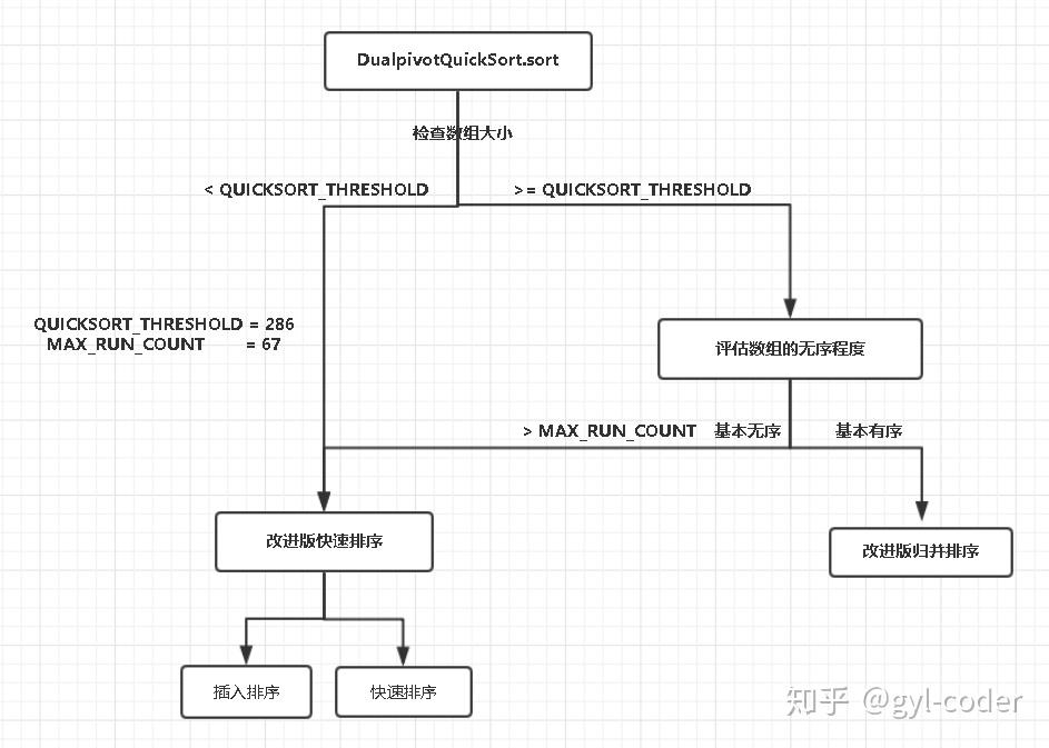
实现过程:首先检查数组的大小,如果数组比较小(通过跟阈值QUICKSORT_THRESHOLD比较),则直接调用改进后的快速排序完成排序,如果数组较大,接着再评估数组的无序程度,如果这个数组几乎是无序的(通过跟阈值MAX_RUN_COUNT比较),那么同样调用改进后的快速排序算法排序;如果数组基本有序,则采用归并排序算法对数组进行排序。
下面我们来分析具体实现:
14-18行
检查了数组的大小,如果数组大小小于QUICKSORT_THRESHOLD的值,则直接调用改进快排实现排序。阈值QUICKSORT_THRESHOLD的值为286。
20-62行
评估数组的无序程度。
基本思路如下:
对于任意的数组,我们总是可以将其分割成若干个递增或递减的子数组(或者说:拆分成若干个“单调”的子数组),例如:序列 {9, 5, 2, 7, 8, 3, 4} 可以拆分为3个单调子数组:{9, 5, 2}、{7, 8}、{3, 4}, 其中每一个子数组都是单调的,不是递增,就是递减。
定义run数组来存储每一个子数组的开始下标,该部分的for循环体对于递增、递减、相等的子序列进行了处理。29、30行的if分句判定了递增子序列;31-35行的else if分句处理的递减序列,同时将递减序列转化为递增序列;36-43的else分句处理了相等的序列。
PS:这里需要注意的是在上面进行递增递减判定的时候,判定条件中都包含了等于因此,只有当前面的if和else if的情况都不成立时,后面的else分句才会执行。例如:序列{1, 2, 3, 3, 3, 3},以及{3, 2, 1, 1, 1}划分后仅为1个子序列,就是它本身;而序列{1, 2, 3, 2, 2, 2}则会被划分成2个子序列:{1, 2, 3} 和 {2, 2, 2}。
46-53行
给出了评估数组无序程度的指标。即考察划分出的子序列的个数,即run数组的大小,如果run数组元素个数大于常量 MAX_RUN_COUNT, 那么认为整个数组基本上是无序的,此时调用改进的快排算法排序,后面的代码不再执行;否则,程序认为整个数组基本上是有序的,继续执行下面的代码,利用归并排序算法完成排序。常量程序MAX_RUN_COUNT定义其值为67。
55-58行
给run数组的末尾添加了一个“哨兵”元素,这个元素的值为right+1,代表一个空的子序列。这里又分为两种情况:如果原数组在划分后最后一个元素独自为一个子序列,那么在27-43行的循环执行完毕后,run数组的最后一个元素的值为right,此时须有再添加一个代表空序列的哨兵元素;如果划分后,原数组中的最后一个元素并不是独自为一个子序列,那么27-43行的循环执行完毕后,run数组的最后一个元素的值就是right+1,此时run数组的最后一个元素已经是哨兵,就不需要再添加了。
程序执行到这里,意味着程序认为数组基本上是有序的,采用归并排序算法进行排序,这个哨兵元素的作用接下来会有体现。
56-62行
给出了另一种特殊情况,即整个数组划分后就只有1个单调子序列,那么说明数组本身就是有序的,不需要再执行其他操作,程序结束。
64-110行
该部分程序对划分好的数据进行了二路归并排序。
64-86行
是一个初始化的操作,88-109行是归并排序的主体,循环的每一轮迭代都将数组a中的两个相邻的单调子序列“归并”为一个新的单调子序列,并存储在数组b中。90行开始的内层的for循环成对的归并数组a中的单调子序列。
循环中的每轮迭代将两个相邻的单调子序列进行归并,第一个子序列的范围是run[k-2] - run[i-1], 第二个子序列的范围是run[k-1] - run[k],内层循环每次迭代都将k增加2。同时last变量记录了归并得到的新的子序列的个数,同时更新run数组的内容。
PS:这里需要注意,如果a数组中的子序列个数是奇数,那么最后一个子序列就无法进行配对、归并操作,此时,直接将这个子序列复制到b中。 代码是101-106行完成了这个工作。
每轮迭代以后,子序列的数目都会减少,因此,反复地进行迭代归并后,最终会使得整个数组只包含1个单调递增的子序列,此时整个数组排序完成。因此,每轮迭代后,交换a、b指针,继续执行下一轮迭代时,同样对a数组进行归并,存储在b数组中。就这样,利用a和b代表的存储空间反复的进行归并,就可以完成数组的排序。107-108行的代码完成了交换a和b指针的工作。
初始情况下,a和b指针一个指向原数组,另一个指向辅助空间。下面的if语句则根据需要的迭代次数对a和b指针的指向进行指定,确保在迭代归并结束以后,排好序的数组依旧在调用函数之前的存储空间内。这里的代码还检查了辅助空间的大小是否足够,如果不够,则重新申请内存。
最后,对于90行的循环还有一个问题,当处理a数组的最后一对单调子序列的归并操作时,此时,hi的值已经超出了run数组的大小,即k值已经越界,为了避免这种情况的发生,我们在run数组的末尾添加了一个“哨兵”元素,这样就保证了在循环过程中不会发生数组越界的异常。
快速排序(改进版)
在上面的排序代码中的16、40、51行调用了DualPivotQuicksort类中的另一个排序方法,该方法的实现机理是基于对于传统快速排序的改进,在待排序数据基本无序时被调用。
/**
* Sorts the specified range of the array by Dual-Pivot Quicksort.
*
* @param a the array to be sorted
* @param left the index of the first element, inclusive, to be sorted
* @param right the index of the last element, inclusive, to be sorted
* @param leftmost indicates if this part is the leftmost in the range
*/
private static void sort(int[] a, int left, int right, boolean leftmost) {
int length = right - left + 1;
// Use insertion sort on tiny arrays
if (length < INSERTION_SORT_THRESHOLD) {
if (leftmost) {
/*
* Traditional (without sentinel) insertion sort,
* optimized for server VM, is used in case of
* the leftmost part.
*/
for (int i = left, j = i; i < right; j = ++i) {
int ai = a[i + 1];
while (ai < a[j]) {
a[j + 1] = a[j];
if (j-- == left) {
break;
}
}
a[j + 1] = ai;
}
} else {
/*
* Skip the longest ascending sequence.
*/
do {
if (left >= right) {
return;
}
} while (a[++left] >= a[left - 1]);
/*
* Every element from adjoining part plays the role
* of sentinel, therefore this allows us to avoid the
* left range check on each iteration. Moreover, we use
* the more optimized algorithm, so called pair insertion
* sort, which is faster (in the context of Quicksort)
* than traditional implementation of insertion sort.
*/
for (int k = left; ++left <= right; k = ++left) {
int a1 = a[k], a2 = a[left];
if (a1 < a2) {
a2 = a1; a1 = a[left];
}
while (a1 < a[--k]) {
a[k + 2] = a[k];
}
a[++k + 1] = a1;
while (a2 < a[--k]) {
a[k + 1] = a[k];
}
a[k + 1] = a2;
}
int last = a[right];
while (last < a[--right]) {
a[right + 1] = a[right];
}
a[right + 1] = last;
}
return;
}
// Inexpensive approximation of length / 7
int seventh = (length >> 3) + (length >> 6) + 1;
/*
* Sort five evenly spaced elements around (and including) the
* center element in the range. These elements will be used for
* pivot selection as described below. The choice for spacing
* these elements was empirically determined to work well on
* a wide variety of inputs.
*/
int e3 = (left + right) >>> 1; // The midpoint
int e2 = e3 - seventh;
int e1 = e2 - seventh;
int e4 = e3 + seventh;
int e5 = e4 + seventh;
// Sort these elements using insertion sort
if (a[e2] < a[e1]) { int t = a[e2]; a[e2] = a[e1]; a[e1] = t; }
if (a[e3] < a[e2]) { int t = a[e3]; a[e3] = a[e2]; a[e2] = t;
if (t < a[e1]) { a[e2] = a[e1]; a[e1] = t; }
}
if (a[e4] < a[e3]) { int t = a[e4]; a[e4] = a[e3]; a[e3] = t;
if (t < a[e2]) { a[e3] = a[e2]; a[e2] = t;
if (t < a[e1]) { a[e2] = a[e1]; a[e1] = t; }
}
}
if (a[e5] < a[e4]) { int t = a[e5]; a[e5] = a[e4]; a[e4] = t;
if (t < a[e3]) { a[e4] = a[e3]; a[e3] = t;
if (t < a[e2]) { a[e3] = a[e2]; a[e2] = t;
if (t < a[e1]) { a[e2] = a[e1]; a[e1] = t; }
}
}
}
// Pointers
int less = left; // The index of the first element of center part
int great = right; // The index before the first element of right part
if (a[e1] != a[e2] && a[e2] != a[e3] && a[e3] != a[e4] && a[e4] != a[e5]) {
/*
* Use the second and fourth of the five sorted elements as pivots.
* These values are inexpensive approximations of the first and
* second terciles of the array. Note that pivot1 <= pivot2.
*/
int pivot1 = a[e2];
int pivot2 = a[e4];
/*
* The first and the last elements to be sorted are moved to the
* locations formerly occupied by the pivots. When partitioning
* is complete, the pivots are swapped back into their final
* positions, and excluded from subsequent sorting.
*/
a[e2] = a[left];
a[e4] = a[right];
/*
* Skip elements, which are less or greater than pivot values.
*/
while (a[++less] < pivot1);
while (a[--great] > pivot2);
/*
* Partitioning:
*
* left part center part right part
* +--------------------------------------------------------------+
* | < pivot1 | pivot1 <= && <= pivot2 | ? | > pivot2 |
* +--------------------------------------------------------------+
* ^ ^ ^
* | | |
* less k great
*
* Invariants:
*
* all in (left, less) < pivot1
* pivot1 <= all in [less, k) <= pivot2
* all in (great, right) > pivot2
*
* Pointer k is the first index of ?-part.
*/
outer:
for (int k = less - 1; ++k <= great; ) {
int ak = a[k];
if (ak < pivot1) { // Move a[k] to left part
a[k] = a[less];
/*
* Here and below we use "a[i] = b; i++;" instead
* of "a[i++] = b;" due to performance issue.
*/
a[less] = ak;
++less;
} else if (ak > pivot2) { // Move a[k] to right part
while (a[great] > pivot2) {
if (great-- == k) {
break outer;
}
}
if (a[great] < pivot1) { // a[great] <= pivot2
a[k] = a[less];
a[less] = a[great];
++less;
} else { // pivot1 <= a[great] <= pivot2
a[k] = a[great];
}
/*
* Here and below we use "a[i] = b; i--;" instead
* of "a[i--] = b;" due to performance issue.
*/
a[great] = ak;
--great;
}
}
// Swap pivots into their final positions
a[left] = a[less - 1]; a[less - 1] = pivot1;
a[right] = a[great + 1]; a[great + 1] = pivot2;
// Sort left and right parts recursively, excluding known pivots
sort(a, left, less - 2, leftmost);
sort(a, great + 2, right, false);
/*
* If center part is too large (comprises > 4/7 of the array),
* swap internal pivot values to ends.
*/
if (less < e1 && e5 < great) {
/*
* Skip elements, which are equal to pivot values.
*/
while (a[less] == pivot1) {
++less;
}
while (a[great] == pivot2) {
--great;
}
/*
* Partitioning:
*
* left part center part right part
* +----------------------------------------------------------+
* | == pivot1 | pivot1 < && < pivot2 | ? | == pivot2 |
* +----------------------------------------------------------+
* ^ ^ ^
* | | |
* less k great
*
* Invariants:
*
* all in (*, less) == pivot1
* pivot1 < all in [less, k) < pivot2
* all in (great, *) == pivot2
*
* Pointer k is the first index of ?-part.
*/
outer:
for (int k = less - 1; ++k <= great; ) {
int ak = a[k];
if (ak == pivot1) { // Move a[k] to left part
a[k] = a[less];
a[less] = ak;
++less;
} else if (ak == pivot2) { // Move a[k] to right part
while (a[great] == pivot2) {
if (great-- == k) {
break outer;
}
}
if (a[great] == pivot1) { // a[great] < pivot2
a[k] = a[less];
/*
* Even though a[great] equals to pivot1, the
* assignment a[less] = pivot1 may be incorrect,
* if a[great] and pivot1 are floating-point zeros
* of different signs. Therefore in float and
* double sorting methods we have to use more
* accurate assignment a[less] = a[great].
*/
a[less] = pivot1;
++less;
} else { // pivot1 < a[great] < pivot2
a[k] = a[great];
}
a[great] = ak;
--great;
}
}
}
// Sort center part recursively
sort(a, less, great, false);
} else { // Partitioning with one pivot
/*
* Use the third of the five sorted elements as pivot.
* This value is inexpensive approximation of the median.
*/
int pivot = a[e3];
/*
* Partitioning degenerates to the traditional 3-way
* (or "Dutch National Flag") schema:
*
* left part center part right part
* +-------------------------------------------------+
* | < pivot | == pivot | ? | > pivot |
* +-------------------------------------------------+
* ^ ^ ^
* | | |
* less k great
*
* Invariants:
*
* all in (left, less) < pivot
* all in [less, k) == pivot
* all in (great, right) > pivot
*
* Pointer k is the first index of ?-part.
*/
for (int k = less; k <= great; ++k) {
if (a[k] == pivot) {
continue;
}
int ak = a[k];
if (ak < pivot) { // Move a[k] to left part
a[k] = a[less];
a[less] = ak;
++less;
} else { // a[k] > pivot - Move a[k] to right part
while (a[great] > pivot) {
--great;
}
if (a[great] < pivot) { // a[great] <= pivot
a[k] = a[less];
a[less] = a[great];
++less;
} else { // a[great] == pivot
/*
* Even though a[great] equals to pivot, the
* assignment a[k] = pivot may be incorrect,
* if a[great] and pivot are floating-point
* zeros of different signs. Therefore in float
* and double sorting methods we have to use
* more accurate assignment a[k] = a[great].
*/
a[k] = pivot;
}
a[great] = ak;
--great;
}
}
/*
* Sort left and right parts recursively.
* All elements from center part are equal
* and, therefore, already sorted.
*/
sort(a, left, less - 1, leftmost);
sort(a, great + 1, right, false);
}
}该算法的实现了“双枢轴快速排序”,它是经典快速排序算法的变体。
算法的基本思路是:如果数组的数据量较少,则执行插入排序以达到更好的效果,如果数据量较大,那么确定数组的5个分位点,选择一个或两个分位点作为“枢轴”,然后根据快速排序的思想进行排序。
12-72行
这一部分对数组进行插入排序。如果数组长度小于阈值INSERTION _SORT_THRESHOLD,,程序认为这是一个小规模的数组,采用插入排序算法进行处理,后面的代码不再执行;否则,程序执行快速排序算法处理。这里的阈值INSERTION _SORT_THRESHOLD程序定义其值为47。
这一部分对于插入排序也给出了一种改进的方案,基本思路是:每次迭代过程中同时完成两个元素的插入排序,代码的注释给出了该算法的名称—— pair insertion sort,中文可以译为“双插入排序”。代码中第15-29行为经典插入排序算法的实现,32-70行为双插入排序算法的实现。
下面简要说明双插入排序算法的思路。
48-63行的循环代码中用a1和a2两个变量存储每次迭代时要完成排序的两个相邻的元素。首先确保a1和a2的大小关系是a1≥a2。然后利用变量k遍历a1和a2之前的元素,找到第一个小于a1的元素的位置,确定a1的位置,54-57行的while循环完成了这一步骤;由于a2≤a1,所以a2的位置一定在a1之前,因此,确定了a1的位置后,k继续遍历,此时的步骤和普通的插入排序是完全相同的,59-62行的代码完成了这一步骤。
对于双插入排序,有一种特殊情况,如果原数组的元素格式是奇数的话,那么最后一个元素就没有元素与其配对完成插入排序,因此,还需要额外进行一次插入排序来完成排序,这里的处理步骤和经典插入排序也和经典插入排序是完全相同的,65-79行的代码完成了这个处理过程。
另外,为了提高算法效率,在算法开始前,我们可以跳过数组前面已经有序的部分,从第一个无序的元素开始遍历、插入,31-38行的代码完成了这个初始化过程。
需要注意的是,48-63行的代码中,对于变量k的值没有进行数组边界检查,根据给出的代码注释,现有的程序设计思路下,即使不对k变量进行数组越界的检查,也一定不会发生异常。
### 74-108行
如果数组比较大,那么就要采用快速排序的算法来处理。这一部分程序对于快速排序算法的进行确定了分位点。分为点的确定思路是将数组长度划分为7等份,然后确定5个分割点为3/14分位点、5/14分位点、中点、9/14分位点以及11/14分位点,程序中分别记为:e1、e2、e3、e4、e5。
确定分位点后, 90-107行代码,对于5个分位点的元素进行了排序。
109-336行
快速排序算法的主体。具体实现分为两种情况。
第一种
如果前面得到的5个分位点的值各不相同,那么就选择e2和e4分为点作为快速排序的“枢轴”,采用双枢轴快速排序算法进行排序;否则,选择e3,作为枢轴,进行快速排序,这里虽然仅有一个枢轴点,但也和经典的快速排序算法有一定的区别。
为了提高算法效率,131-135行程序在迭代开始前对于数组进行了预处理,找出已经有序的第一部分和第三部分,迭代从第一个失序的元素开始。
第二种
第一种方法为5个分位点个各不相同的处理情况,而对于5个分位点如果存在两个分位点的值相同,程序给出了另一种策略,此时不再使用双枢轴,而是仅选择 pivot = e3 分位点作为唯一的枢轴点,不同于经典快速排序算法的是,这种情况下,算法依旧将数组划分为三个部分:小于pivot的部分、等于pivot的部分以及大于pivot的部分。
具体过程双枢轴快速排序中有详细介绍。