NetworkX——谈一谈Python中网络的构建、绘制与最短路搜索

近期在某研究中,需要实现类似于百度地图的“智行”与滴滴打车的“公交车”功能,主要目的是将多种出行方式进行组合。这里面就涉及到了两个网络层,层间通过某些节点可以做到互通,而层内则可以全通。仔细想想,还是有些复杂的。于是一开始,我花了两天时间认认真真的写了算法,然后在开始动手撸代码的时候,才发现原来Python上早有包可以做了。这个包就是做复杂网络的基础包——NETWOTKX。
好了,直接进入正题。目前研究思路是很清晰的。有两个网络层,姑且设为A层与B层,每个层间属性各不相同,如出行成本、出行距离等。但层内是完全互通的,即只要在一层内,任意两个点都是有路到达的。
层间也是可以相通的,但不能随意互通,而需要通过某些换乘点来完成层间的换乘。因此实际上,可以把这个理解为三个网络层:A层,B层,和换乘层。每个层的属性各不相同,需要分别构造,在构造完成后,再进行合并,即可完成整体网络的构建了。在完成整体网络的构建后,后面的工作就交给NETWORKX好了。根据不同的权重寻找最短路径,输出路径成本及路径节点,绘制效果图,都是一行代码的事情。
下面结合代码分别进行介绍。
单层网络构建
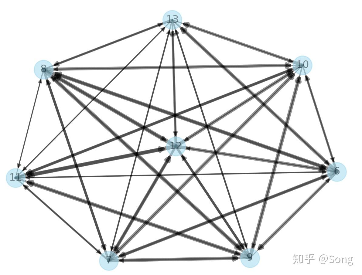
在第一步中,我们对两个网络层分别进行构造。每一个DataFrame中,至少需要三列,分别表示起点、终点与该路径权重。我们这里构造了四列,后两列从不同角度来表示权重。
from_pandas_edgelist可以直接把DF转化为NX所需要的网络结构。最终绘制结果如下:

#!/usr/bin/env python3
# -*- coding: utf-8 -*-

import os
import numpy as np
import pandas as pd
import math
import matplotlib.pyplot as plt
from pylab import *
import seaborn as sns
import random
import pylab

os.chdir('/Users/husonghua/Desktop/EV+SUBWAY/')

####################Build the raw network####################
# Subway network
# We suppose that there are five station in the metro system. (From 1 to 5)
SB_NUM = 5
SB_NET = pd.DataFrame({'SUB_O': np.repeat(range(1, SB_NUM + 1), SB_NUM),
					   'SUB_D': list(range(1, SB_NUM + 1)) * SB_NUM,
					   'SUB_T': [random.randint(1, 100) for x in range(SB_NUM * SB_NUM)],
					   'SUB_M': [random.randint(5, 10) for x in range(SB_NUM * SB_NUM)]})

# Build subway graph and plot
G = nx.from_pandas_edgelist(SB_NET, 'SUB_O', 'SUB_D', ['SUB_T', 'SUB_M'], create_using=nx.DiGraph())
# Plot
pos = nx.spring_layout(G)
pylab.figure(1)
nx.draw(G, pos, with_labels=True, node_size=500, node_color="skyblue", node_shape="o", alpha=0.5,
		width=SB_NET['SUB_T'] / 10)
# edge_labels = dict([((u, v,), d['SUB_T']) for u, v, d in G.edges(data=True)])
# nx.draw_networkx_edge_labels(G, pos, edge_labels=edge_labels, font_color='red')

# EV network
# We suppose that there are eight station in the EV system. (From 6 to 13)
EV_NUM = 8
EV_NET = pd.DataFrame({'EV_O': np.repeat(range(SB_NUM + 1, EV_NUM + SB_NUM + 1), EV_NUM),
					   'EV_D': list(range(SB_NUM + 1, EV_NUM + SB_NUM + 1)) * EV_NUM,
					   'EV_T': [random.randint(10, 50) for x in range(EV_NUM * EV_NUM)],
					   'EV_M': [random.randint(20, 50) for x in range(EV_NUM * EV_NUM)]})

# Build EV graph and plot
G = nx.from_pandas_edgelist(EV_NET, 'EV_O', 'EV_D', ['EV_T', 'EV_M'], create_using=nx.DiGraph())
# Plot
pos = nx.spring_layout(G)
pylab.figure(1)
nx.draw(G, pos, with_labels=True, node_size=500, node_color="skyblue", node_shape="o", alpha=0.5,
		width=EV_NET['EV_T'] / 10)
####################Build the raw network####################
网络连接层构建
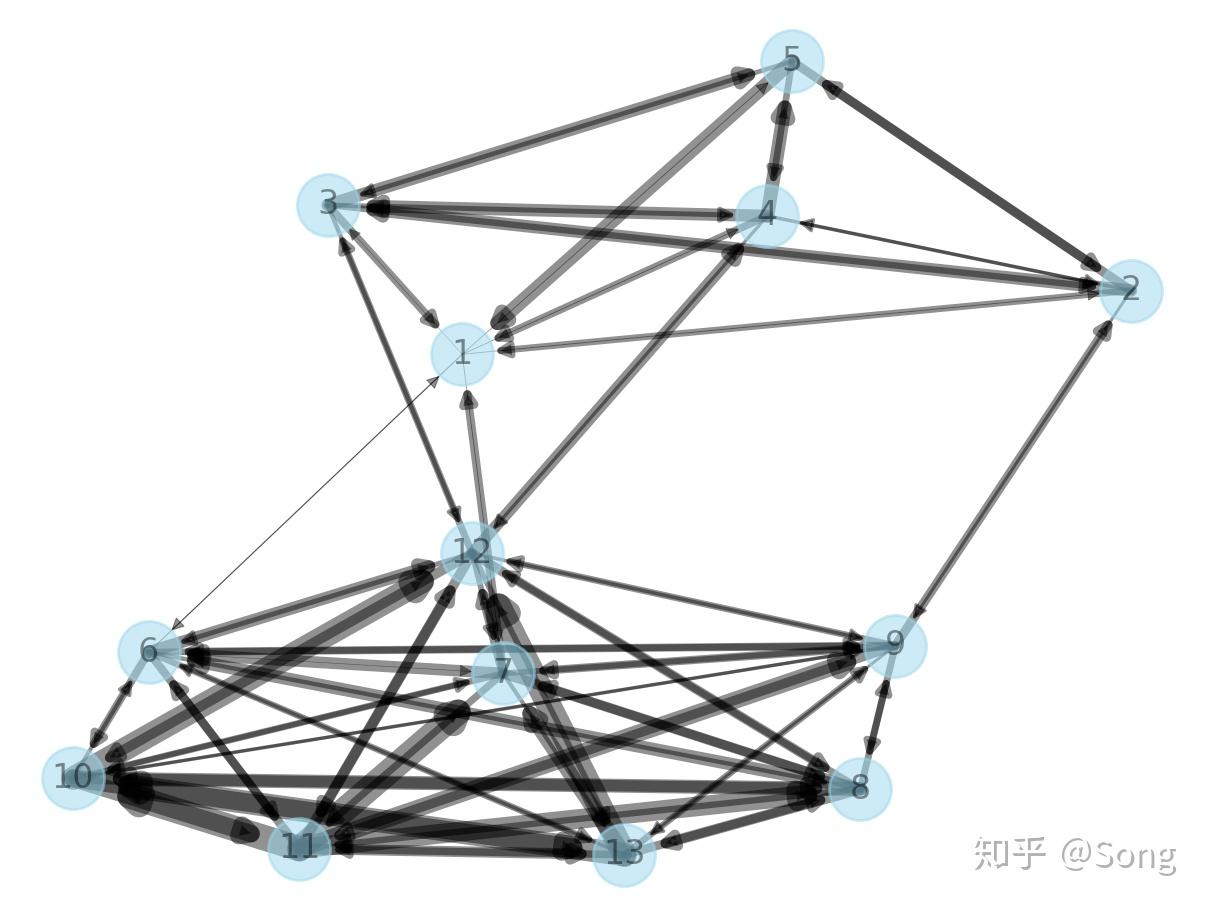
网络连接层的构建其实和之前单层网络的构建方法完全一致,只不过其作用在于连接两个网络,且不能直接互通全连接。最后通过concatenate将三个DF合并为一个(不用concat因为三个DF列名不同)。最后绘制的网络图如下。可以看到明显的两个网络层(1-5)与(6-13),以及两者间的换乘层。

# Adjacency List
# Suppose: 1 --> (6,7); (3,4) --> 12; 2 --> 9
EV_SB = pd.DataFrame({'ADJ_O': [1, 1, 6, 7, 3, 4, 12, 12, 2, 9],
					  'ADJ_D': [6, 7, 1, 1, 12, 12, 3, 4, 9, 2],
					  'ADJ_T': [random.randint(1, 5) for x in range(10)],
					  'ADJ_M': [random.randint(1, 2) for x in range(10)]})

# Merge three network into one
npCombined_Net = np.concatenate([EV_SB.as_matrix(), EV_NET.as_matrix(), SB_NET.as_matrix()], axis=0)
Combined_Net = pd.DataFrame(npCombined_Net, columns=["COM_O", "COM_D", "COM_T", "COM_M"])

# Build graph and plot
G = nx.from_pandas_edgelist(Combined_Net, 'COM_O', 'COM_D', ['COM_T', 'COM_M'], create_using=nx.DiGraph())
# Plot
pos = nx.spring_layout(G)
pylab.figure(1)
nx.draw(G, pos, with_labels=True, node_size=500, node_color="skyblue", node_shape="o", alpha=0.5,
		width=Combined_Net['COM_T'] / 10)
最短路计算与绘制
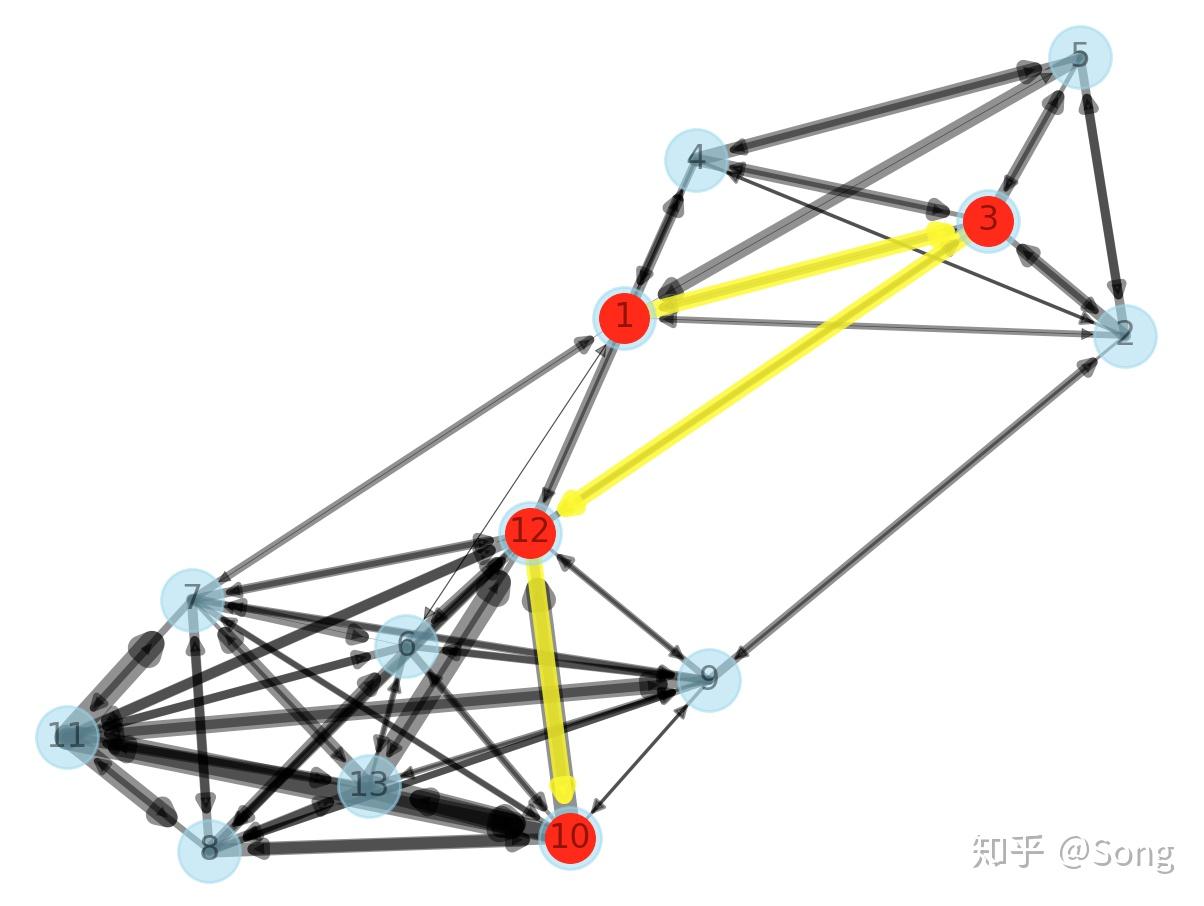
最后一步,就是计算最短路,指定起终点,分布使用shortest_path_length和shortest_path得出最小成本以及最短路径编号。然后再利用NX进行绘制。大功告成。比如从编号1到编号10,是需要跨层的,而最短路选择了3和12作为中间节点进行换乘,符合需求。

####################Calculate the shortest path and highlight in graph####################
# Input the O and D
origin_node = 1
destination_node = 10
# Calculate the shortest path using the weight of Money or time
distance = nx.shortest_path_length(G, origin_node, destination_node, weight='COM_M')
path = nx.shortest_path(G, source=origin_node, target=destination_node, weight='COM_M')
# Plot
# Plot the whole raw network
G = nx.from_pandas_edgelist(Combined_Net, 'COM_O', 'COM_D', ['COM_T', 'COM_M'], create_using=nx.DiGraph())
pos = nx.spring_layout(G)
pylab.figure(1)
nx.draw(G, pos, with_labels=True, node_size=500, node_color="skyblue", node_shape="o", alpha=0.5,
		width=Combined_Net['COM_T'] / 10)
# Plot the shortest path
path_edges = list(zip(path, path[1:]))
nx.draw_networkx_nodes(G, pos, nodelist=path, node_color='r')
nx.draw_networkx_edges(G, pos, edgelist=path_edges, edge_color='yellow', width=6, alpha=0.8)
####################Calculate the shortest path and highlight in graph####################
总结
掉包诚可耻,效率价更高。通过NX,难点则转移到了前面的网络构建及参数确定的环节了,而最短路的寻优算法不再成为羁绊。当然,调包都只是停留在技术层面,要到理论层面,还是自己扎扎实实的造轮子的好。