
【SSD算法】史上最全代码解析-核心篇

前言
最近,在回顾之前看过的论文和代码时,看到SSD的代码和思想非常适合从基础层面去理解目标检测的各种思想。
因此,我决定写一个 详细、全面、细致 的代码解析,希望能够让更多的人能无师自通,能够很好的了解如何结合paper去实现代码。
SSD Pytorch版本的代码来至于 Amdegroot 的 Pytorch 版本。
目录
- 网络模型
- VGG Backbone
- Extra Layers
- Multi-box Layers
- SSD 模型类
- 先验框生成
- 损失函数
- L2 正则化
- 训练处理
- 位置坐标转换
- IOU计算
- 位置编码和解码
- 先验框匹配
- NMS抑制
- Detection函数
网络模型
⛳️ 整个网络是由三大部分组成:
- VGG Backbone
- Extra Layers
- Multi-box Layers
VGG Backbone
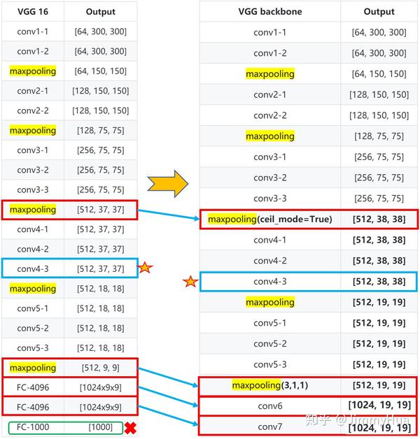
✔️ 根据SSD的论文描述,作者采用了vgg16的部分网络作为基础网络,在5层网络后,丢弃全连接,改为两个卷积网络,分别为:1024x3x3、1024x1x1。
✏️ 值得注意:
1. conv4-1前面一层的maxpooling的ceil_mode=True,使得输出为 38x38;
2. Conv4-3网络是需要输出多尺度的网络层;
3. Conv5-3后面的一层maxpooling参数为(kernel_size=3, stride=1, padding=1),不进行下采样。
网络层次图:

网络代码:
def vgg(cfg, i, batch_norm=False):
'''
该代码参考vgg官网的代码
'''
    layers = []
    in_channels = i
    for v in cfg:
        # 正常的 max_pooling
        if v == 'M':
            layers += [nn.MaxPool2d(kernel_size=2, stride=2)]

        # ceil_mode = True, 上采样使得 channel 75-->38
        elif v == 'C':
            layers += [nn.MaxPool2d(kernel_size=2, stride=2, ceil_mode=True)]
        else:
            conv2d = nn.Conv2d(in_channels, v, kernel_size=3, padding=1)
            if batch_norm:
                layers += [conv2d, nn.BatchNorm2d(v), nn.ReLU(inplace=True)]
            else:
                layers += [conv2d, nn.ReLU(inplace=True)]
            # update in_channels
            in_channels = v

    # max_pooling (3,3,1,1)
    pool5 = nn.MaxPool2d(kernel_size=3, stride=1, padding=1)
    # 新添加的网络层 1024x3x3
    conv6 = nn.Conv2d(512, 1024, kernel_size=3, padding=6, dilation=6)

    # 新添加的网络层 1024x1x1
    conv7 = nn.Conv2d(1024, 1024, kernel_size=1)

    # 结合到整体网络中
    layers += [pool5, conv6,
               nn.ReLU(inplace=True), conv7, nn.ReLU(inplace=True)]
    return layers

# 代码测试
if __name__ == "__main__":
    base = {
    '300': [64, 64, 'M', 128, 128, 'M', 256, 256, 256, 'C', 512, 512, 512, 'M',
            512, 512, 512],
    '512': [],
    }
    vgg = nn.Sequential(*vgg(base['300'], 3))
    x = torch.randn(1,3,300,300)
    print(vgg(x).shape)  #(1, 1024, 19, 19)
不同的写法
def vggs():
    '''
    调用torchvision.models里面的vgg,
    修改对应的网络层,同样可以得到目标的backbone。
    '''
    vgg16 = models.vgg16()
    vggs = vgg16.features
    vggs[16] = nn.MaxPool2d(2, 2, 0, 1, ceil_mode=True)
    vggs[-1] = nn.MaxPool2d(3, 1, 1, 1, ceil_mode=False)
    conv6 = nn.Conv2d(512, 1024, kernel_size=3, padding=6, dilation=6)
    conv7 = nn.Conv2d(1024, 1024, kernel_size=1)
    '''
    方法一:
    '''
    #vggs= nn.Sequential(feature, conv6, nn.ReLU(inplace=True), conv7, nn.ReLU(inplace=True))

    '''
    方法二:
    '''
    vggs.add_module('31',conv6)
    vggs.add_module('32',nn.ReLU(inplace=True))
    vggs.add_module('33',conv7)
    vggs.add_module('34',nn.ReLU(inplace=True))
    #print(vggs)
    x = torch.randn(1,3,300,300)
    print(vggs(x).shape)

    return vgg
输出网络结构:
Sequential(
  (0): Conv2d(3, 64, kernel_size=(3, 3), stride=(1, 1), padding=(1, 1))
  (1): ReLU(inplace)
  (2): Conv2d(64, 64, kernel_size=(3, 3), stride=(1, 1), padding=(1, 1))
  (3): ReLU(inplace)
  (4): MaxPool2d(kernel_size=2, stride=2, padding=0, dilation=1, ceil_mode=False)
  (5): Conv2d(64, 128, kernel_size=(3, 3), stride=(1, 1), padding=(1, 1))
  (6): ReLU(inplace)
  (7): Conv2d(128, 128, kernel_size=(3, 3), stride=(1, 1), padding=(1, 1))
  (8): ReLU(inplace)
  (9): MaxPool2d(kernel_size=2, stride=2, padding=0, dilation=1, ceil_mode=False)
  (10): Conv2d(128, 256, kernel_size=(3, 3), stride=(1, 1), padding=(1, 1))
  (11): ReLU(inplace)
  (12): Conv2d(256, 256, kernel_size=(3, 3), stride=(1, 1), padding=(1, 1))
  (13): ReLU(inplace)
  (14): Conv2d(256, 256, kernel_size=(3, 3), stride=(1, 1), padding=(1, 1))
  (15): ReLU(inplace)
  (16): MaxPool2d(kernel_size=2, stride=2, padding=0, dilation=1, ceil_mode=True)
  (17): Conv2d(256, 512, kernel_size=(3, 3), stride=(1, 1), padding=(1, 1))
  (18): ReLU(inplace)
  (19): Conv2d(512, 512, kernel_size=(3, 3), stride=(1, 1), padding=(1, 1))
  (20): ReLU(inplace)
  (21): Conv2d(512, 512, kernel_size=(3, 3), stride=(1, 1), padding=(1, 1))
  (22): ReLU(inplace)
  (23): MaxPool2d(kernel_size=2, stride=2, padding=0, dilation=1, ceil_mode=False)
  (24): Conv2d(512, 512, kernel_size=(3, 3), stride=(1, 1), padding=(1, 1))
  (25): ReLU(inplace)
  (26): Conv2d(512, 512, kernel_size=(3, 3), stride=(1, 1), padding=(1, 1))
  (27): ReLU(inplace)
  (28): Conv2d(512, 512, kernel_size=(3, 3), stride=(1, 1), padding=(1, 1))
  (29): ReLU(inplace)
  (30): MaxPool2d(kernel_size=3, stride=1, padding=1, dilation=1, ceil_mode=False)
  (31): Conv2d(512, 1024, kernel_size=(3, 3), stride=(1, 1), padding=(6, 6), dilation=(6, 6))
  (32): ReLU(inplace)
  (33): Conv2d(1024, 1024, kernel_size=(1, 1), stride=(1, 1))
  (34): ReLU(inplace)
)
Extra Layers
作者为了后续的多尺度提取,在VGG Backbone后面添加了卷积网络。

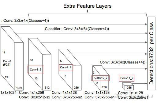
网络层次:
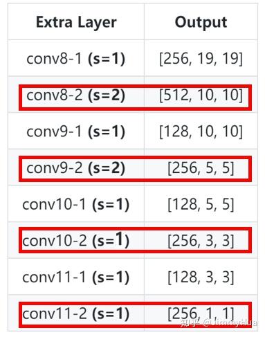
PS: 红框的网络需要进行多尺度分析,输入到multi-box网络。
网络代码:
def add_extras(cfg, i, batch_norm=False):
    '''
    为后续多尺度提取,增加网络层
    '''
    layers = []
    # 初始输入通道为 1024
    in_channels = i
    # flag 用来选择 kernel_size= 1 or 3
    flag = False
    for k,v in enumerate(cfg):
        if in_channels != 'S':
            if v == 'S':
                layers += [nn.Conv2d(in_channels, cfg[k+1],
                                    kernel_size=(1,3)[flag], stride=2, padding=1)]
            else:
                layers += [nn.Conv2d(in_channels, v, kernel_size=(1, 3)[flag])]

            flag = not flag # 反转flag

        in_channels = v # 更新 in_channels

    return layers
# 代码测试
if __name__ == "__main__":
    extras = {
    '300': [256, 'S', 512, 128, 'S', 256, 128, 256, 128, 256],
    '512': [],
    }
    layers = add_extras(extras['300'], 1024)
    print(nn.Sequential(*layers))
输出:
Sequential(
  (0): Conv2d(1024, 256, kernel_size=(1, 1), stride=(1, 1))
  (1): Conv2d(256, 512, kernel_size=(3, 3), stride=(2, 2), padding=(1, 1))
  (2): Conv2d(512, 128, kernel_size=(1, 1), stride=(1, 1))
  (3): Conv2d(128, 256, kernel_size=(3, 3), stride=(2, 2), padding=(1, 1))
  (4): Conv2d(256, 128, kernel_size=(1, 1), stride=(1, 1))
  (5): Conv2d(128, 256, kernel_size=(3, 3), stride=(1, 1))
  (6): Conv2d(256, 128, kernel_size=(1, 1), stride=(1, 1))
  (7): Conv2d(128, 256, kernel_size=(3, 3), stride=(1, 1))
)
Multi-box Layers
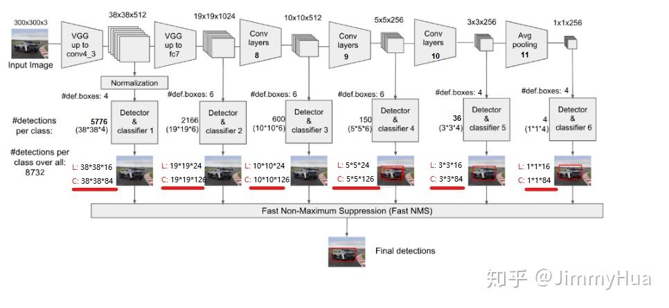
SSD一共有6层多尺度提取的网络,每层分别对 loc 和 conf 进行卷积,得到相应的输出。
网络层次:

网络代码:
def multibox(vgg, extra_layers, cfg, num_classes):
    '''
    Args:
        vgg: 修改fc后的vgg网络
        extra_layers: 加在vgg后面的4层网络
        cfg: 网络参数,eg:[4, 6, 6, 6, 4, 4]
        num_classes: 类别,VOC为 20+背景=21
    Return:
        vgg, extra_layers
        loc_layers: 多尺度分支的回归网络
        conf_layers: 多尺度分支的分类网络
    '''
    loc_layers = []
    conf_layers = []
    vgg_layer = [21, -2]
    # 第一部分,vgg 网络的 Conv2d-4_3(21层), Conv2d-7_1(-2层)
    for k, v in enumerate(vgg_layer):
        # 回归 box*4(坐标)
        loc_layers += [nn.Conv2d(vgg[v].out_channels, cfg[k]*4, kernel_size=3, padding=1)]
        # 置信度 box*(num_classes)
        conf_layers += [nn.Conv2d(vgg[v].out_channels, cfg[k]*num_classes, kernel_size=3, padding=1)]

    # 第二部分,cfg从第三个开始作为box的个数,而且用于多尺度提取的网络分别为1,3,5,7层
    for k, v in enumerate(extra_layers[1::2],2):
        # 回归 box*4(坐标)
        loc_layers += [nn.Conv2d(v.out_channels, cfg[k]*4, kernel_size=3, padding=1)]
        # 置信度 box*(num_classes)
        conf_layers += [nn.Conv2d(v.out_channels, cfg[k]*(num_classes), kernel_size=3, padding=1)]

    return vgg, extra_layers, (loc_layers, conf_layers)
if __name__  == "__main__":
    vgg, extra_layers, (l, c) = multibox(vgg(base['300'], 3),
                                         add_extras(extras['300'], 1024),
                                         [4, 6, 6, 6, 4, 4], 21)
    print(nn.Sequential(*l))
    print('---------------------------')
    print(nn.Sequential(*c))
输出:
'''
loc layers:
'''
Sequential(
  (0): Conv2d(512, 16, kernel_size=(3, 3), stride=(1, 1), padding=(1, 1))
  (1): Conv2d(1024, 24, kernel_size=(3, 3), stride=(1, 1), padding=(1, 1))
  (2): Conv2d(512, 24, kernel_size=(3, 3), stride=(1, 1), padding=(1, 1))
  (3): Conv2d(256, 24, kernel_size=(3, 3), stride=(1, 1), padding=(1, 1))
  (4): Conv2d(256, 16, kernel_size=(3, 3), stride=(1, 1), padding=(1, 1))
  (5): Conv2d(256, 16, kernel_size=(3, 3), stride=(1, 1), padding=(1, 1))
)
---------------------------
'''
conf layers:
'''
Sequential(
  (0): Conv2d(512, 84, kernel_size=(3, 3), stride=(1, 1), padding=(1, 1))
  (1): Conv2d(1024, 126, kernel_size=(3, 3), stride=(1, 1), padding=(1, 1))
  (2): Conv2d(512, 126, kernel_size=(3, 3), stride=(1, 1), padding=(1, 1))
  (3): Conv2d(256, 126, kernel_size=(3, 3), stride=(1, 1), padding=(1, 1))
  (4): Conv2d(256, 84, kernel_size=(3, 3), stride=(1, 1), padding=(1, 1))
  (5): Conv2d(256, 84, kernel_size=(3, 3), stride=(1, 1), padding=(1, 1))
)
SSD 模型类
根据上述的三个网络层结合,结合后面提到的 prior_box和detection方法可以,完整的写出SSD的类。
class SSD(nn.Module):
    '''
    Args:
        phase: string, 可选"train" 和 "test"
        size: 输入网络的图片大小
        base: VGG16的网络层(修改fc后的)
        extras: 用于多尺度增加的网络
        head: 包含了各个分支的loc和conf
        num_classes: 类别数

    return:
        output: List, 返回loc, conf 和 候选框
    '''
    def __init__(self, phase, size, base, extras, head, num_classes):
        super(SSD, self).__init__()
        self.phase = phase
        self.size = size
        self.num_classes = num_classes
        # 配置config
        self.cfg = (coco, voc)[num_classes == 21]
        # 初始化先验框
        self.priorbox = PriorBox(self.cfg)
        self.priors = self.priorbox.forward()
        # basebone 网络
        self.vgg = nn.ModuleList(base)
        # conv4_3后面的网络,L2 正则化
        self.L2Norm = L2Norm(512, 20)
        self.extras = nn.ModuleList(extras)
        # 回归和分类网络
        self.loc = nn.ModuleList(head[0])
        self.conf = nn.ModuleList(head[1])

        if phase == 'test':
        '''
            # 预测使用
            self.softmax = nn.Softmax(dim=-1)
            self.detect = Detect(num_classes, 200, 0.01, 0.045)
        '''
            pass

    def forward(self, x):
        sources, loc ,conf = [], [], []

        # vgg网络到conv4_3
        for i in range(23):
            x = self.vgg[i](x)
        # l2 正则化
        s = self.L2Norm(x)
        sources.append(s)

        # conv4_3 到 fc
        for i in range(23, len(self.vgg)):
            x = self.vgg[i](x)
        sources.append(x)

        # extras 网络
        for k,v in enumerate(self.extras):
            x = F.relu(v(x), inplace=True)
            # 把需要进行多尺度的网络输出存入 sources
            if k%2 == 1:
                sources.append(x)

        # 多尺度回归和分类网络
        for (x, l, c) in zip(sources, self.loc, self.conf):
            loc.append(l(x).permute(0, 2, 3, 1).contiguous())
            conf.append(c(x).permute(0, 2, 3, 1).contiguous())

        loc = torch.cat([o.view(o.size(0), -1) for o in loc], 1)
        conf = torch.cat([o.view(o.size(0), -1) for o in conf], 1)

        if self.phase == 'test':
        '''
        # 预测使用
            output = self.detect(
                    # loc 预测
                    loc.view(loc.size(0), -1, 4),
                    # conf 预测
                    self.softmax(conf.view(conf.size(0), -1, self.num_classes)),
                    # default box
                    self.priors.type(type(x.data)),
                    )
        '''
            pass
        else:
            output = (
                # loc的输出,size:(batch, 8732, 4)
                loc.view(loc.size(0), -1 ,4),
                 # conf的输出,size:(batch, 8732, 21)
                conf.view(conf.size(0), -1, self.num_classes),
                # 生成所有的候选框 size([8732, 4])
                self.priors,
                )
#            print(type(x.data))
#            print((self.priors.type(type(x.data))).shape)
        return output

    # 加载模型参数
    def load_weights(self, base_file):
        print('Loading weights into state dict...')
        self.load_state_dict(torch.load(base_file))
        print('Finished!')
使用build_ssd()封装函数,增加可读性:
def build_ssd(phase, size=300, num_classes=21):
    # 判断phase是否为满足的条件
    if phase != "test" and phase !="train":
        print("Error: Phase:" + phase +" not recognized!\n")
        return
    # 判断size是否为满足的条件
    if size != 300:
        print("Error: currently only size=300 is supported!")
        return

    # 调用multibox,生成vgg,extras,head
    base_, extras_, head_ = multibox(vgg(base[str(size)], 3),
                                     add_extras(extras[str(size)], 1024),
                                     mbox['300'], num_classes,
                                     )
    return SSD(phase, size, base_, extras_, head_, num_classes)

# 调试函数
if __name__ == '__main__':
    ssd = build_ssd('train')
    x = torch.randn(1, 3, 300, 300)
    y = ssd(x)
    print("Loc    shape: ", y[0].shape)
    print("Conf   shape: ", y[1].shape)
    print("Priors shape: ", y[2].shape)
输出:
Loc    shape:  torch.Size([1, 8732, 4])
Conf   shape:  torch.Size([1, 8732, 21])
Priors shape:  torch.Size([8732, 4])
先验框生成
✔️ SSD从Conv4_3开始,一共提取了6个特征图,其大小分别为 (38,38),(19,19),(10,10),(5,5),(3,3),(1,1),但是每个特征图上设置的先验框数量不同。
✔️ 先验框的设置,包括尺度(或者说大小)和长宽比两个方面。对于先验框的尺度,其遵守一个线性递增规则:随着特征图大小降低,先验框尺度线性增加:
s_{k}=s_{m i n}+\frac{s_{m a x}-s_{m i n}}{m-1}(k-1), k \in[1, m]
其中:
- M 指特征图个数,但是为5,因为第一层(Conv4_3)是单独设置的;
- s_k 表示先验框大小相对于图片的比例;
- s_{min} 和 s_{max} 表示比例的最小值与最大值,paper里面取 0.2 和 0.9。
1、对于第一个特征图,它的先验框尺度比例设置为 s_{min}/2=0.1 ,则其尺度为 300 \times 0.1=30 ;
2、对于后面的特征图,先验框尺度按照上面公式线性增加,但是为了方便计算,先将尺度比例先扩大100倍,此时增长步长为:
\delta = \left\lfloor\frac{\left\lfloor s_{m a x} \times 100\right\rfloor-\left\lfloor s_{m i n} \times 100\right\rfloor}{m-1}\right\rfloor= 17
3、根据上面的公式,则有:
s_k = s_{min} \times 100 + \delta
s_k \in\left\{20, 37, 54, 71, 88\right\}
4、将上面的值除以100,然后再乘回原图的大小300,再综合第一个特征图的先验框尺寸,则可得各个特征图的先验框尺寸为:
s_k \in\left\{30, 60, 111, 162, 213, 264\right\}
5、先验框的长宽比一般设置为:
a_{r} \in\left\{1,2,3, \frac{1}{2}, \frac{1}{3}\right\}
6、根据面积和长宽比可得先验框的宽度和高度:
w_{k}^{a}=s_{k} \sqrt{a_{r}}, \space h_{k}^{a}=s_{k} / \sqrt{a_{r}}
7、默认情况下,每个特征图会有一个 a_{r}=1 且尺度为 s_{k} 的先验框,除此之外,还会设置一个尺度为 s_{k}^{\prime}=\sqrt{s_{k} s_{k+1}} 且 a_{r}=1 的先验框,这样每个特征图都设置了两个长宽比为1但大小不同的正方形先验框;
8、最后一个特征图需要参考一个虚拟 s_{m+1}=300 \times (88+17) / 100=315 来计算 s_{m}
9、因此,每个特征图一共有 6 个先验框 \left\{1,2,3, \frac{1}{2}, \frac{1}{3}, 1^{\prime}\right\} ,但是在实现时,Conv4_3,Conv10_2和Conv11_2层仅使用4个先验框,它们不使用长宽比为 3, \frac{1}{3} 的先验框;
10、每个单元的先验框的中心点分布在各个单元的中心,即:
\left(\frac{i+0.5}{\left|f_{k}\right|}, \frac{j+0.5}{\left|f_{k}\right|}\right), i, j \in\left[0,\left|f_{k}\right|\right)
其中 \left|f_{k}\right| 为特征图的大小。
因此,SSD 先验框共个数:
num_priors = 38x38x4+19x19x6+10x10x6+5x5x6+3x3x4+1x1x4=8732代码:
class PriorBox(object):
    """
    1、计算先验框,根据feature map的每个像素生成box;
    2、框的中个数为: 38×38×4+19×19×6+10×10×6+5×5×6+3×3×4+1×1×4=8732
    3、 cfg: SSD的参数配置,字典类型
    """
    def __init__(self, cfg):
        super(PriorBox, self).__init__()
        self.img_size = cfg['img_size']
        self.feature_maps = cfg['feature_maps']
        self.min_sizes = cfg['min_sizes']
        self.max_sizes = cfg['max_sizes']
        self.steps = cfg['steps']
        self.aspect_ratios = cfg['aspect_ratios']
        self.clip = cfg['clip']
        self.version = cfg['name']
        self.variance = cfg['variance']

    def forward(self):
        mean = [] #用来存放 box的参数

        # 遍多尺度的 map: [38, 19, 10, 5, 3, 1]
        for k, f in enumerate(self.feature_maps):
            # 遍历每个像素
            for i, j in product(range(f), repeat=2):
                # k-th 层的feature map 大小
                f_k = self.img_size/self.steps[k]
                # 每个框的中心坐标
                cx = (i+0.5)/f_k
                cy = (j+0.5)/f_k
                '''
                当 ratio==1的时候,会产生两个 box
                '''
                # r==1, size = s_k, 正方形
                s_k = self.min_sizes[k]/self.img_size
                mean += [cx, cy, s_k, s_k]

                # r==1, size = sqrt(s_k * s_(k+1)), 正方形
                s_k_plus = self.max_sizes[k]/self.img_size
                s_k_prime = sqrt(s_k * s_k_plus)
                mean += [cx, cy, s_k_prime, s_k_prime]

                '''
                当 ratio != 1 的时候,产生的box为矩形
                '''
                for r in self.aspect_ratios[k]:
                    mean += [cx, cy, s_k * sqrt(r), s_k / sqrt(r)]
                    mean += [cx, cy, s_k / sqrt(r), s_k * sqrt(r)]

        # 转化为 torch
        boxes = torch.tensor(mean).view(-1, 4)
        # 归一化,把输出设置在 [0,1]
        if self.clip:
            boxes.clamp_(max=1, min=0)

        return boxes

# 调试代码
if __name__ == "__main__":
    # SSD300 CONFIGS
    voc = {
        'num_classes': 21,
        'lr_steps': (80000, 100000, 120000),
        'max_iter': 120000,
        'feature_maps': [38, 19, 10, 5, 3, 1],
        'img_size': 300,
        'steps': [8, 16, 32, 64, 100, 300],
        'min_sizes': [30, 60, 111, 162, 213, 264],
        'max_sizes': [60, 111, 162, 213, 264, 315],
        'aspect_ratios': [[2], [2, 3], [2, 3], [2, 3], [2], [2]],
        'variance': [0.1, 0.2],
        'clip': True,
        'name': 'VOC',
    }
    box = PriorBox(voc)
    print('Priors box shape:', box.forward().shape)
    print('Priors box:\n',box.forward())
输出:
Priors box shape: torch.Size([8732, 4])
Priors box:
tensor([[0.0133, 0.0133, 0.1000, 0.1000],
        [0.0133, 0.0133, 0.1414, 0.1414],
        [0.0133, 0.0133, 0.1414, 0.0707],
        ...,
        [0.5000, 0.5000, 0.9612, 0.9612],
        [0.5000, 0.5000, 1.0000, 0.6223],
        [0.5000, 0.5000, 0.6223, 1.0000]])
损失函数
✔️ SSD的损失函数包括两部分的加权:
- 位置损失函数 L_{loc}
- 置信度损失函数 L_{conf}
整个损失函数为:
L(x, c, l, g)=\frac{1}{N}\left(L_{c o n f}(x, c)+\alpha L_{l o c}(x, l, g)\right)
其中:
- N 是先验框的正样本数量;
- c 为类别置信度预测值;
- l 为先验框的所对应边界框的位置预测值;
- g 为ground truth的位置参数。
1. 对于位置损失函数:
针对所有的正样本,采用 Smooth L1 Loss, 位置信息都是 encode 之后的位置信息。
\operatorname{smooth}_{L_{1}}(x)=\left\{\begin{array}{ll}{0.5 x^{2}} & {\text { if }|x|<1} \\ {|x|-0.5} & {\text { otherwise }}\end{array}\right.
2. 对于置信度损失函数:
首先需要使用 hard negative mining 将正负样本按照 1:3 的比例把负样本抽样出来,抽样的方法是:
思想: 针对所有batch的confidence,按照置信度误差进行降序排列,取出前top_k个负样本。
编程:
- Reshape所有batch中的conf
batch_conf = conf_data.view(-1, self.num_classes)- 置信度误差越大,实际上就是预测背景的置信度越小。
- 把所有conf进行logsoftmax处理(均为负值),预测的置信度越小,则logsoftmax越小,取绝对值,则
|logsoftmax|越大,降序排列-logsoftmax,取前top_k的负样本。
详细分析:
这里借用logsoftmax的思想:
\begin{aligned} \log \left(\frac{e^{x_{j}}}{\sum_{i=1}^{n} e^{x_{i}}}\right) &=\log \left(e^{x_{j}}\right)-\log \left(\sum_{i=1}^{n} e^{x_{i}}\right) \\ &=x_{j}-\log \left(\sum_{i=1}^{n} e^{x_{i}}\right) \end{aligned}
为了防止数值溢出,可以把问题转化为:
\begin{aligned} \log \operatorname{Sum} \operatorname{Exp}\left(x_{1} \ldots x_{n}\right) &=\log \left(\sum_{i=1}^{n} e^{x_{i}}\right) \\ &=\log \left(\sum_{i=1}^{n} e^{x_{i}-c} e^{c}\right) \\ &=\log \left(e^{c} \sum_{i=1}^{n} e^{x_{i}-c}\right) \\ &=\log \left(\sum_{i=1}^{n} e^{x_{i}-c}\right)+\log \left(e^{c}\right) \\ &=\log \left(\sum_{i=1}^{n} e^{x_{i}-c}\right)+c \end{aligned}
上述变换的关键在于,我们引入了一个不牵涉log或exp函数的常数项c。
现在我们只需为 c 选择一个在所有情形下有效的良好的值,结果发现,$max(x_1…x_n)$很不错。
由此我们可以构建对数softmax的新表达式:
\begin{aligned} \log \left(\operatorname{Softmax}\left(x_{j}, x_{1} \ldots x_{n}\right)\right) &=x_{j}-\log \operatorname{Sum} \operatorname{Exp}\left(x_{1} \ldots x_{n}\right) \\ &=x_{j}-\log \left(\sum_{i=1}^{n} e^{x_{i}-c}\right)-c \end{aligned}
因此,可以把排序的函数定义为:
conflogP = \operatorname{Softmax}\left(x_{j}, x_{1} \ldots x_{n}\right) - x_j
python代码:
logSumExp的表示为:
def log_sum_exp(x):
    x_max = x.detach().max()
    return torch.log(torch.sum(torch.exp(x-x_max), 1, keepdim=True))+x_max
conf_logP 表示为:
conf_logP = log_sum_exp(batch_conf) - batch_conf.gather(1, conf_t.view(-1, 1))排除正样本
conf_logP.view(batch, -1) # shape[b, M]
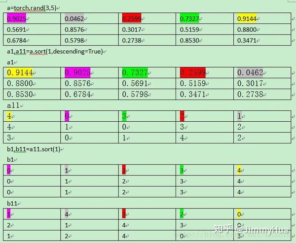
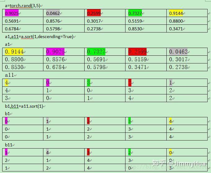
conf_logP[pos] = 0 # 把正样本排除,剩下的就全是负样本,可以进行抽样两次sort,能够得到每个元素在降序排列中的位置idx_rank
_, index = conf_logP.sort(1, descending=True)
_, idx_rank = index.sort(1)
可以参考如下表:
后续,就可以筛选出所需的负样本,配合正样本求出conf的cross entropy。
完整loss代码
# -*- coding: utf-8 -*-
"""
Created on Tue Aug 13 10:52:36 2019

@author: Jimmy Hua
"""
import torch
import torch.nn as nn
import torch.nn.functional as F
from vgg_backbone import voc
from box_utils import match, log_sum_exp

class MultiBoxLoss(nn.Module):
    def __init__(self, num_classes, overlap_thresh, neg_pos, use_gpu=False):
        super(MultiBoxLoss, self).__init__()
        self.use_gpu =  use_gpu
        self.num_classes = num_classes
        self.threshold = overlap_thresh
        self.negpos_ratio = neg_pos
        self.variance = voc['variance']

    def forward(self, pred, targets):
        '''
        Args:
            pred: A tuple, 包含 loc(编码钱的位置信息), conf(类别), priors(先验框);
                  loc_data: shape[b,M,4];
                  conf_data: shape[b,M,num_classes];
                  priors: shape[M,4];

            targets: 真实的boxes和labels,shape[b,num_objs,5];
        '''
        loc_data, conf_data, priors = pred
        batch = loc_data.size(0)  #batch
        num_priors = priors[:loc_data.size(1), :].size(0) # 先验框个数

        # 获取匹配每个prior box的 ground truth
        # 创建 loc_t 和 conf_t 保存真实box的位置和类别
        loc_t = torch.Tensor(batch, num_priors, 4)
        conf_t = torch.LongTensor(batch, num_priors)

        for idx in range(batch):
            truths = targets[idx][:, :-1].detach() # ground truth box信息
            labels = targets[idx][:, -1].detach()  # ground truth conf信息
            defaults = priors.detach()     # priors的 box 信息

            # 匹配 ground truth
            match(self.threshold, truths, defaults,
                  self.variance, labels, loc_t, conf_t, idx)

        # use gpu
        if self.use_gpu:
            loc_t = loc_t.cuda()
            conf_t = conf_t.cuda()

        pos = conf_t > 0 # 匹配中所有的正样本mask,shape[b,M]

        # Localization Loss,使用 Smooth L1
        # shape[b,M]-->shape[b,M,4]
        pos_idx = pos.unsqueeze(2).expand_as(loc_data)
        loc_p = loc_data[pos_idx].view(-1,4)  # 预测的正样本box信息
        loc_t = loc_t[pos_idx].view(-1,4)     # 真实的正样本box信息
        loss_l = F.smooth_l1_loss(loc_p, loc_t) # Smooth L1 损失

        '''
        Target;
            下面进行hard negative mining
        过程:
            1、 针对所有batch的conf,按照置信度误差(预测背景的置信度越小,误差越大)进行降序排列;
            2、 负样本的label全是背景,那么利用log softmax 计算出logP,
               logP越大,则背景概率越低,误差越大;
            3、 选取误差交大的top_k作为负样本,保证正负样本比例接近1:3;
        '''
        # shape[b*M,num_classes]
        batch_conf = conf_data.view(-1, self.num_classes)
        # 使用logsoftmax,计算置信度,shape[b*M, 1]
        conf_logP = log_sum_exp(batch_conf) - batch_conf.gather(1, conf_t.view(-1, 1))

        # hard Negative Mining
        conf_logP = conf_logP.view(batch, -1) # shape[b, M]
        conf_logP[pos] = 0 # 把正样本排除,剩下的就全是负样本,可以进行抽样

        # 两次sort排序,能够得到每个元素在降序排列中的位置idx_rank
        _, index = conf_logP.sort(1, descending=True)
        _, idx_rank = index.sort(1)

        # 抽取负样本
        # 每个batch中正样本的数目,shape[b,1]
        num_pos = pos.long().sum(1, keepdim=True)
        num_neg = torch.clamp(self.negpos_ratio*num_pos, max= pos.size(1)-1)
        neg = idx_rank < num_neg # 抽取前top_k个负样本,shape[b, M]

        # shape[b,M] --> shape[b,M,num_classes]
        pos_idx = pos.unsqueeze(2).expand_as(conf_data)
        neg_idx = neg.unsqueeze(2).expand_as(conf_data)

        # 提取出所有筛选好的正负样本(预测的和真实的)
        conf_p = conf_data[(pos_idx+neg_idx).gt(0)].view(-1, self.num_classes)
        conf_target = conf_t[(pos+neg).gt(0)]

        # 计算conf交叉熵
        loss_c = F.cross_entropy(conf_p, conf_target)

        # 正样本个数
        N = num_pos.detach().sum().float()

        loss_l /= N
        loss_c /= N

        return loss_l, loss_c

# 调试代码使用
if __name__ == "__main__":
    loss = MultiBoxLoss(21, 0.5, 3)
    p = (torch.randn(1,100,4), torch.randn(1,100,21), torch.randn(100,4))
    t = torch.randn(1, 10, 4)
    tt = torch.randint(20, (1,10,1))
    t = torch.cat((t,tt.float()), dim=2)
    l, c = loss(p, t)
    # 随机randn,会导致g_wh出现负数,此时结果会变成 nan
    print('loc loss:', l)
    print('conf loss:', c)
输出:
loc loss: tensor(11.9424)
conf loss: tensor(2.0487)
L2 正则化
✔️ VGG网络的conv4_3特征图大小38x38,网络层靠前,norm较大,需要加一个L2 Normalization,以保证和后面的检测层差异不是很大。
L2 norm 的公式如下:
\hat{\mathbf{x}}=\frac{\mathbf{x}}{\|\mathbf{x}\|_{2}} \space\space\space\cdots\text{(1)}
其中:
\mathbf{x}=\left(x_{1} \cdots x_{d}\right) \|\mathbf{x}\|_{2}=\left(\sum_{i=1}^{d}\left|x_{i}\right|^{2}\right)^{1 / 2}\space\space\space\cdots\text{(2)}
注意,如果我们不按比例缩小学习范围,简单地对一个层的每个输入进行标准化就会改变该层的规模,并且会减慢速度学习,因此需要引入一个scaling paraneter \gamma_{i} ,对于每一个通道,l2 norm 变为:
y_{i}=\gamma_{i} \hat{x}_{i}\space\space\space\cdots\text{(3)}
通常,scale 值设为10或20,效果比较好。
代码:
class L2Norm(nn.Module):
    '''
    conv4_3特征图大小38x38,网络层靠前,norm较大,需要加一个L2 Normalization,
    以保证和后面的检测层差异不是很大,具体可以参考: ParseNet。
    '''
    def __init__(self, n_channels, scale):
        super(L2Norm, self).__init__()
        self.n_channels = n_channels
        self.gamma = scale or None
        self.eps = 1e-10
        # 将一个不可训练的类型Tensor转换成可以训练的类型 parameter
        self.weight = nn.Parameter(torch.Tensor(self.n_channels))
        self.reset_parameters()

    # 初始化参数
    def reset_parameters(self):
        nn.init.constant_(self.weight, self.gamma)

    def forward(self, x):
        # 计算 x 的2范数,参考公式 (2)
        norm = x.pow(2).sum(dim=1, keepdim=True).sqrt() # shape[b,1,38,38]

        # 参考公式 (1)
        x = x / norm   # shape[b,512,38,38]

        # 扩展self.weight的维度为shape[1,512,1,1],然后参考公式
        out = self.weight[None,...,None,None] * x

        return out

# 测试代码
if __name__ == "__main__":
    x = torch.randn(1, 512, 38, 38)
    l2norm = L2Norm(512, 20)
    out = l2norm(x)
    print('L2 norm :', out.shape)
输出:
L2 norm : torch.Size([1, 512, 38, 38])训练处理
位置坐标转换
✔️ Bounding Box的位置表示方式有两种:
A: (x_{min}, \space y_{min}, \space x_{max}, \space y_{max})
B: (x_{c}, \space y_{c}, \space w, \space h)
代码:
# B --> A
def point_form(boxes):
    '''
    把 prior_box (cx, cy, w, h)转化为(xmin, ymin, xmax, ymax)
    '''
    return torch.cat((boxes[:, :2] - boxes[:, 2:]/2,      # xmin, ymin
                      boxes[:, :2] + boxes[:, 2:]/2,), 1) # xmax, ymax

# A --> B
def center_size(boxes):
    '''
    把 prior_box (xmin, ymin, xmax, ymax) 转化为 (cx, cy, w, h)
    '''
    return torch.cat((boxes[:, :2] + boxes[:, 2:])/2,      # cx, cy
                      (boxes[:, 2:] - boxes[:, :2],), 1)    # w, h
IOU计算
✔️ IOU的原称为Intersection over Union,也就是两个box区域的交集比上并集,下面的示意图就很好理解,用于确定两个框的位置像素距离。

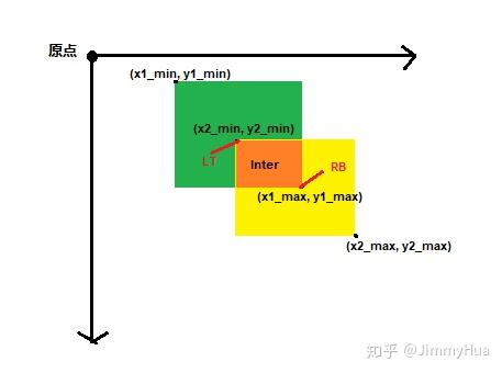
思路:(注意维度一致)
- 首先计算两个box左上角点坐标的最大值和右下角坐标的最小值
- 然后计算交集面积
- 最后把交集面积除以对应的并集面积
代码:
def iou(box_a, box_b):
    '''
    IOU = A∩B/A∪B
    Args:
        box_a: Ground truth bounding box: shape[N, 4]
        box_b: Priors bounding box: shape[M, 4]
    '''
    N = box_a.size(0)
    M = box_b.size(0)

    # 左上角,选出最大值
    LT = torch.max(
            box_a[:, :2].unsqueeze(1).expand(N, M, 2), #(N,2)-->(N,1,2)-->(N,M,2)
            box_b[:, :2].unsqueeze(0).expand(N, M, 2), #(M,2)-->(M,1,2)-->(N,M,2)
            )
    # 右上角
    RB = torch.min(
            box_a[:, 2:].unsqueeze(1).expand(N, M, 2), #(N,2)-->(N,1,2)-->(N,M,2)
            box_b[:, 2:].unsqueeze(0).expand(N, M, 2), #(M,2)-->(M,1,2)-->(N,M,2)
            )
    wh = RB - LT
    wh[wh < 0] = 0 # 两个box没有重叠区域

    inter = wh[:, :, 0] * wh[:, :, 1] # A∩B

    # box_a和box_b的面积
    area_a = (box_a[:, 2]-box_a[:, 0]) * (box_a[:, 3]-box_a[:, 1]) #(N,)
    area_b = (box_b[:, 2]-box_b[:, 0]) * (box_b[:, 3]-box_b[:, 1]) #(M,)

    # 把面积的shape扩展为inter一样的(N,M)
    area_a = area_a.unsqueeze(1).expand_as(inter)
    area_b = area_b.unsqueeze(0).expand_as(inter)

    # iou
    iou = inter / (area_a + area_b - inter)

    return iou

# 测试代码
if __name__ == "__main__":
    box_a = torch.Tensor([[2,1,4,3]])
    box_b = torch.Tensor([[3,2,5,4]])
    print('IOU = ',iou(box_a, box_b))
输出:
IOU = tensor([[0.1429]])位置编码和解码
✔️ 根据论文的描述,预测和真实的边界框是有一个转换关系的,具体如下:
- 先验框位置 d=(d^{cx},\space d^{cy}, \space d^{w}, \space d^{h})
- 真实框位置 g=(g^{cx},\space g^{cy}, \space g^{w}, \space g^{h})
- variance 用于调整检测值
编码: 得到预测框相对于default box的偏移量 l 。
\hat{g}_{j}^{cx}=(g_{j}^{cx}-d_{i}^{cx})/d_{i}^{w}/variance[0]
\hat{g}_{j}^{cy}=(g_{j}^{cy}-d_{i}^{cy})/d_{i}^{h}/variance[1]
\hat{g}_{j}^{w}=log(\frac{g_{j}^{w}}{d_{i}^{w}})/variance[2]
\hat{g}_{j}^{h}=log(\frac{g_{j}^{h}}{d_{i}^{h}})/variance[3]
代码:
def encode(matched, priors, variances):
    '''
    将来至于priorbox的差异编码到ground truth box中
    Args:
        matched: 每个prior box 所匹配的ground truth,
                 Shape[M,4],坐标(xmin,ymin,xmax,ymax)
        priors: 先验框box, shape[M,4],坐标(cx, cy, w, h)
        variances: 方差,list(float)
    '''
    # 编码中心坐标cx, cy
    g_cxcy = (matched[:, :2] + matched[:, 2:])/2 -priors[:, :2]
    g_cxcy /= (priors[:, 2:] * variances[0]) #shape[M,2]

    # 防止出现log出现负数,从而使loss为 nan
    eps = 1e-5

    # 编码宽高w, h
    g_wh = (matched[:, 2:] - matched[:, :2]) / priors[:, 2:]
    g_wh = torch.log(g_wh + eps) / variances[1]   #shape[M,2]

    return torch.cat([g_cxcy, g_wh], 1)    #shape[M,4]
解码: 从预测值 l 中得到边界框的真实值。
{g_{\text { predict }}^{c x}=d^{w} *\left(\text { variance }[0] * l^{c x}\right)+d^{c x}}
{g_{\text { predict }}^{c y}=d^{h} *\left(\text { variance }[1] * l^{c y}\right)+d^{c y}}
{g_{\text { predict }}^{w}=d^{w} \exp \left(\text { variance }[2] * l^{w}\right)}
{g_{\text { predict }}^{h}=d^{h} \exp \left(\text { variance }[3] * l^{h}\right)}
代码:
def decode(loc, priors, variances):
    '''
    对应encode,解码预测的位置信息
    '''
    boxes = torch.cat((priors[:, :2] + loc[:, :2] * variances[0] * priors[:, 2:],
                       priors[:, 2:] * torch.exp(loc[:, 2:] * variances[1])),1)

    # 转化坐标为 (xmin, ymin, xmax, ymax)类型
    boxes = point_form(boxes)

    return boxes
先验框匹配
✔️ 在训练过程中,首先需要确定训练图片中的 ground truth 与哪一个先验框来进行匹配,与之匹配的先验框所对应的边界框将负责预测它。
✔️ SSD的先验框和ground truth匹配原则主要两点: 1. 对于图片中的每个gt,找到与其IOU最大的先验框,该先验框与其匹配,这样可以保证每个gt一定与某个prior匹配。 2. 对于剩余未匹配的priors,若某个gt的IOU大于某个阈值(一般0.5),那么该prior与这个gt匹配。
注意点:
- 通常称与gt匹配的prior为正样本,反之,若某一个prior没有与任何一个gt匹配,则为负样本。
2. 某个gt可以和多个prior匹配,而每个prior只能和一个gt进行匹配。
3. 如果多个gt和某一个prior的IOU均大于阈值,那么prior只与IOU最大的那个进行匹配。
代码:
def match(threshold, truths, priors, variances, labels, loc_t, conf_t, idx):
    '''
    Target:
        把和每个prior box 有最大的IOU的ground truth box进行匹配,
        同时,编码包围框,返回匹配的索引,对应的置信度和位置
    Args:
        threshold: IOU阈值,小于阈值设为bg
        truths: ground truth boxes, shape[N,4]
        priors: 先验框, shape[M,4]
        variances: prior的方差, list(float)
        labels: 图片的所有类别,shape[num_obj]
        loc_t: 用于填充encoded loc 目标张量
        conf_t: 用于填充encoded conf 目标张量
        idx: 现在的batch index
    '''
    overlaps = iou(truths, point_form(priors))

    # [1,num_objects] 和每个ground truth box 交集最大的 prior box
    best_prior_overlap, best_prior_idx = overlaps.max(1, keepdim=True)

    # [1,num_priors] 和每个prior box 交集最大的 ground truth box
    best_truth_overlap, best_truth_idx = overlaps.max(0, keepdim=True)

    # squeeze shape
    best_prior_idx.squeeze_(1)       #(N)
    best_prior_overlap.squeeze_(1)   #(N)
    best_truth_idx.squeeze_(0)       #(M)
    best_truth_overlap.squeeze_(0)   #(M)

    # 保证每个ground truth box 与某一个prior box 匹配,固定值为 2 > threshold
    best_truth_overlap.index_fill_(0, best_prior_idx, 2)  # ensure best prior

    # 保证每一个ground truth 匹配它的都是具有最大IOU的prior
    # 根据 best_prior_dix 锁定 best_truth_idx里面的最大IOU prior
    for j in range(best_prior_idx.size(0)):
        best_truth_idx[best_prior_idx[j]] = j

    # 提取出所有匹配的ground truth box, Shape: [M,4]
    matches = truths[best_truth_idx]

    # 提取出所有GT框的类别, Shape:[M]
    conf = labels[best_truth_idx] + 1
    # 把 iou < threshold 的框类别设置为 bg,即为0
    conf[best_truth_overlap < threshold] = 0
    # 编码包围框
    loc = encode(matches, priors, variances)

    # 保存匹配好的loc和conf到loc_t和conf_t中
    loc_t[idx] = loc    # [M,4] encoded offsets to learn
    conf_t[idx] = conf  # [M] top class label for each prior
NMS抑制
✔️ 非极大值抑制(Non-maximum suppression,NMS)是一种去除非极大值的算法,常用于计算机视觉中的边缘检测、物体识别等。
算法流程:
✔️ 给出一张图片和上面许多物体检测的候选框(即每个框可能都代表某种物体),但是这些框很可能有互相重叠的部分,我们要做的就是只保留最优的框。假设有N个框,每个框被分类器计算得到的分数为 S_i , 1\leqslant i \leqslant N 。
- 建造一个存放待处理候选框的集合H,初始化为包含全部N个框;建造一个存放最优框的集合M,初始化为空集。
- 将所有集合 H 中的框进行排序,选出分数最高的框 m,从集合 H 移到集合 M;
- 遍历集合 H 中的框,分别与框 m 计算交并比(Interection-over-union,IoU),如果高于某个阈值(一般为0~0.5),则认为此框与 m 重叠,将此框从集合 H 中去除。
- 回到第2步进行迭代,直到集合 H 为空。集合 M 中的框为我们所需。
示例:
比如人脸识别的一个例子

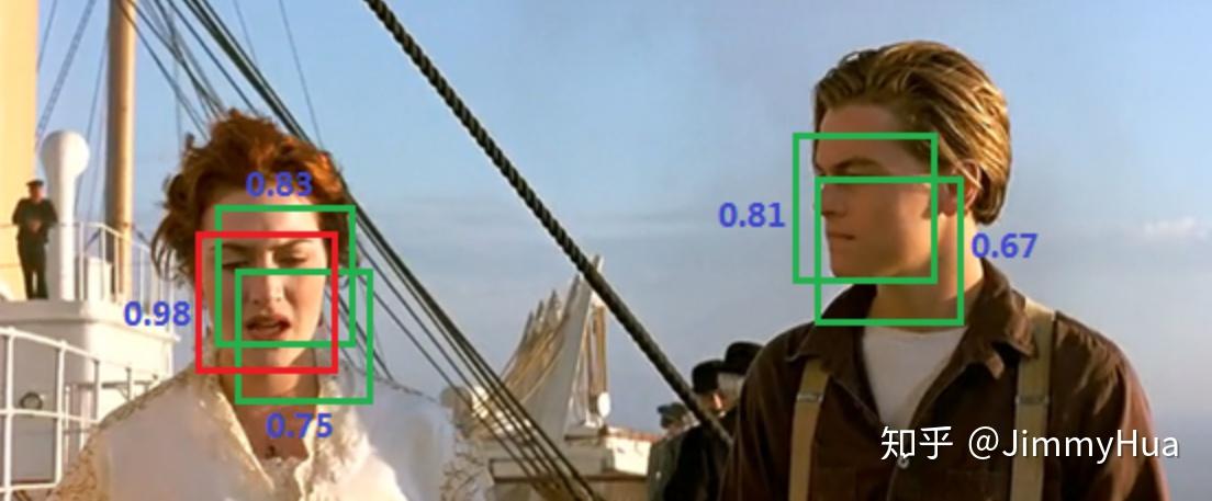
已经识别出了5个候选框,但是我们只需要最后保留两个人脸。
首先选出分数最大的框(0.98),然后遍历剩余框,计算 IoU,会发现露丝脸上的两个绿框都和 0.98 的框重叠率很大,都要去除。
然后只剩下杰克脸上两个框,选出最大框(0.81),然后遍历剩余框(只剩下0.67这一个了),发现0.67这个框与 0.81 的 IoU 也很大,去除。
至此所有框处理完毕,算法结果:


代码:
✔️ NMS算法一般是为了去掉模型预测后的多余框,其一般设有一个nms_threshold=0.5,具体的实现思路如下:
- 选取这类box中scores最大的哪一个,它的index记为 i ,并保留它;
- 计算
boxes[i]与其余的boxes的IOU值; - 如果其
IOU>0.5了,那么就舍弃这个box(由于可能这两个box表示同一目标,所以保留分数高的哪一个) - 从最后剩余的boxes中,再找出最大scores的哪一个,如此循环往复
def nms(boxes, scores, threshold=0.5, top_k=200):
    '''
    Args:
        boxes: 预测出的box, shape[M,4]
        scores: 预测出的置信度,shape[M]
        threshold: 阈值
        top_k: 要考虑的box的最大个数
    Return:
        keep: nms筛选后的box的新的index数组
        count: 保留下来box的个数
    '''
    keep = scores.new(scores.size(0)).zero_().long()
    x1 = boxes[:, 0]
    y1 = boxes[:, 1]
    x2 = boxes[:, 2]
    y2 = boxes[:, 3]

    area = (x2-x1)*(y2-y1)  # 面积,shape[M]
    _, idx = scores.sort(0, descending=True) # 降序排列scores的值大小
    # 取前top_k个进行nms
    idx = idx[:top_k]

    count = 0

    while idx.numel():
        # 记录最大score值的index
        i = idx[0]
        # 保存到keep中
        keep[count] = i
        # keep 的序号
        count += 1

        if idx.size(0) == 1: # 保留框只剩一个
            break

        idx = idx[1:] # 移除已经保存的index

        # 计算boxes[i]和其他boxes之间的iou
        xx1 = x1[idx].clamp(min=x1[i])
        yy1 = y1[idx].clamp(min=y1[i])
        xx2 = x2[idx].clamp(max=x2[i])
        yy2 = y2[idx].clamp(max=y2[i])

        w = (xx2 - xx1).clamp(min=0)
        h = (yy2 - yy1).clamp(min=0)

        # 交集的面积
        inter = w * h  # shape[M-1]
        iou = inter / (area[i] + area[idx] - inter)

        # iou满足条件的idx
        idx = idx[iou.le(threshold)] # Shape[M-1]

    return keep, count
其中:
- torch.numel(): 表示一个张量总元素的个数
- torch.clamp(min, max): 设置上下限
- tensor.le(x): 返回tensor<=x的判断
Detection函数
✔️ 模型进行测试的时候,需要把预测出的loc和conf输入到detect函数进行nms,最后给出相应的结果。
代码:
class Detect(Function):

    def __init__(self, num_classes, top_k, conf_thresh, nms_thresh):
        self.num_classes = num_classes
        self.top_k = top_k
        self.conf_thresh = conf_thresh
        self.nms_thresh = nms_thresh
        self.variance = cfg['variance']

    def forward(self, loc_data, conf_data, prior_data):
        '''
        Args:
            loc_data: 预测出的loc张量,shape[b,M,4], eg:[b, 8732, 4]
            conf_data: 预测出的置信度,shape[b,M,num_classes], eg:[b, 8732, 21]
            prior_data: 先验框,shape[M,4], eg:[8732, 4]
        '''
        batch = loc_data.size(0)    # batch size
        output = torch.zeros(batch, self.num_classes, self.top_k, 5) # 初始化输出
        conf_preds = conf_data.transpose(2,1)

        # 解码loc的信息,变为正常的bboxes
        for i in range(batch):
            # 解码loc
            decode_boxes = decode(loc_data[i], prior_data, self.variance)
            # 拷贝每个batch内的conf,用于nms
            conf_scores = conf_preds[i].clone()

            # 遍历每一个类别
            for num in range(1, self.num_classes):
                # 筛选掉 conf < conf_thresh 的conf
                c_mask = conf_scores[num].gt(self.conf_thresh)
                scores = conf_scores[num][c_mask]
                # 如果都被筛掉了,则跳入下一类
                if scores.size(0) == 0:
                    continue
                # 筛选掉 conf < conf_thresh 的框
                l_mask = c_mask.unsqueeze(1).expand_as(decode_boxes)
                boxes = decode_boxes[l_mask].view(-1, 4)

                # nms
                ids, count = nms(boxes, scores, self.nms_thresh, self.top_k)
                # nms 后得到的输出拼接
                output[i, num, :count] = torch.cat((
                                            scores[ids[:count]].unsqueeze(1),
                                            boxes[ids[:count]]), 1)

        return output

# 代码测试
if __name__ == "__main__":
    detect = Detect(21, 200, 0.01, 0.5)
    loc_data = torch.randn(1,8732,4)
    conf_data = torch.randn(1,8732,21)
    prior_data = torch.randn(8732, 4)

    out = detect(loc_data, conf_data, prior_data)
    print('Detect output shape:', out.shape)
输出:
Detect output shape: torch.Size([1, 21, 200, 5])补充
后续,会继续补充上《数据篇》,其中包括了目标检测中常见到的各种数据增强方法!
未完待续。。。
❤️❤️❤️
。。。内容续上:
包含SSD数据处理和各种数据增强方法,纯python+opencv实现: